
Ver 1.1(this)/1.4(thermoDraw) DISCLAIMER
The individual processes - constant volume, constant temperature, constant entropy, and constant pressure - can be combined to form theoretical cycles.
Contents
Real world cycles are represents by a sequence of theoretical processes.
We consider theoretical models of engines. The working fluid will be a gas, normally an ideal gas and air, rather than steam which behaves non-ideally and undergoes phase change. This note concerns closed cycles wherein working gas is imagined as being contained in a piston-cylinder or recirculated around the engine. Within real-world internal combustion engines the working gas is mixed with fuel and the mixture burns inside the engine (i.e., inside a piston-cylinder or a chamber feeding a turbine). Within external combustion engines heat is transferred to the engine from its surroundings (in practice creating external irreversibilities). This topic considers idealised cycles with no internal irreversibilities. (Real world cycles that exhibit strong external irreversibilities, owing to friction or gradients of temperature, suffer reduced overall efficiency.)
The complex science and mechanics of real-world engines are imagined as a set of simple processes.
A simple example of an engine cycle is the theoretical Carnot cycle (see Figure 1 on this link) , comprising two isothermal processes and two isentropic processes. The petrol engine offers a further example of an open, internal combustion cycle. There are many websites explaining how the four-stroke cycle works , and, using indicator diagrams in particular, demonstrate the difference between real-world and theoretical cycles . The real-world performance is modelled with complex and costly computer programs, but one get some insight by making big, simplifying assumptions. In essence, we treat the engine as one wherein a mass of air is permanently contained inside a piston-cylinder, and is caused to expand or contract by externally applied heating or cooling. We assume that the air behaves ideally. We also assume:
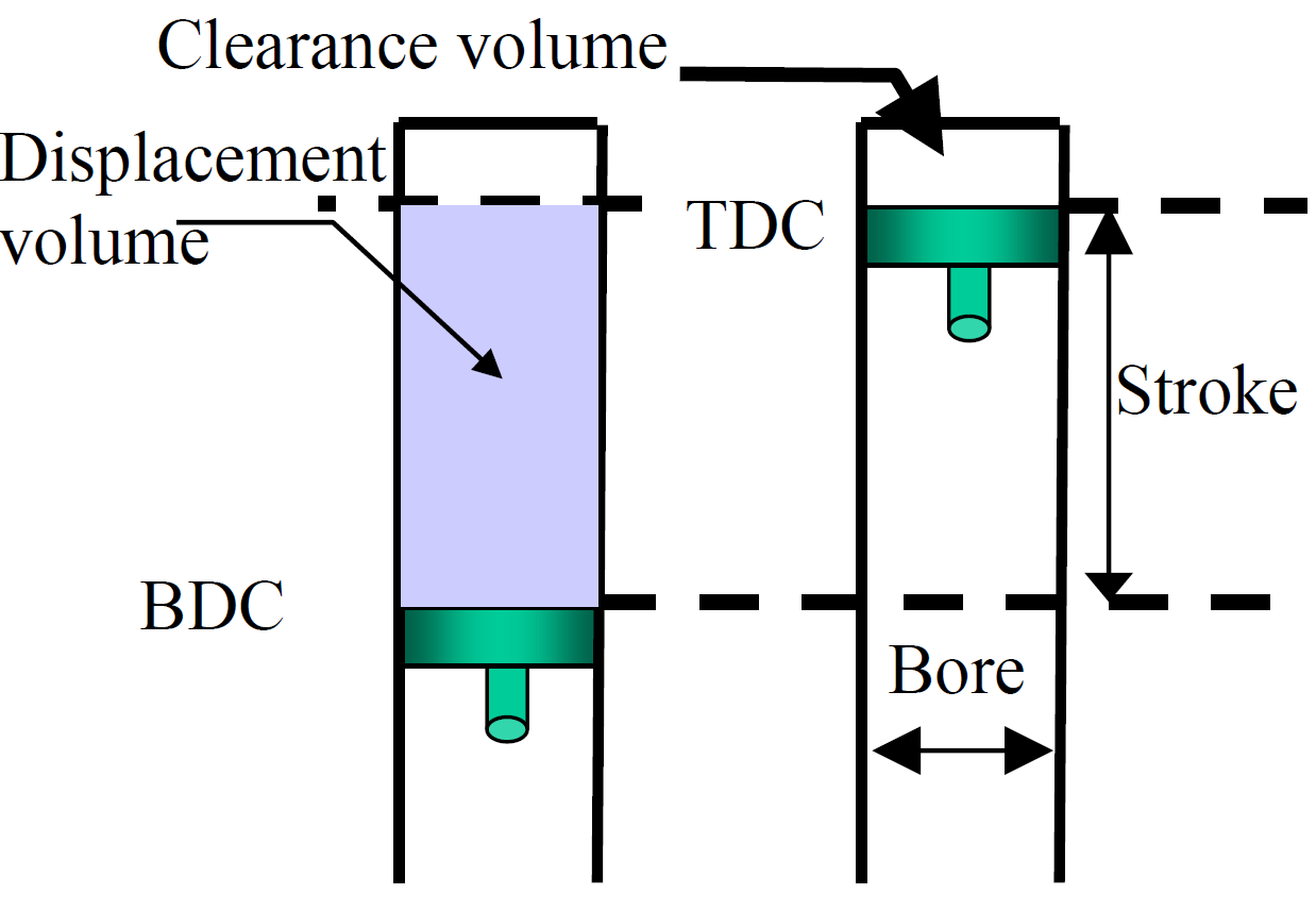
Figure 1. Piston-cylinder showing some technical terms
Important terms for a piston cylinder (Fig. 1) are:
$$ r_v = \frac{V_{max}}{V_{min}} $$ The simple cycles presented here concern only two external heat reservoirs. For such machines, an earlier note presents a specialised form of the First Law
$$ |W_{cyc}| = |Q_H|-|Q_L| $$ where \(Q_H , Q_L\) are heat transfers from hot and cold reservoirs. This leads to a definition of cycle efficiency. $$ \eta_{cyc} = \frac{|W_{cyc}|}{|Q_H|} = 1- \frac{|Q_L|}{|Q_H|} $$
The Otto Cycle is modelled as two constant volume (isochoric) processes of heat transfer and two constant entropy (isentropic) processes of moving boundary work.
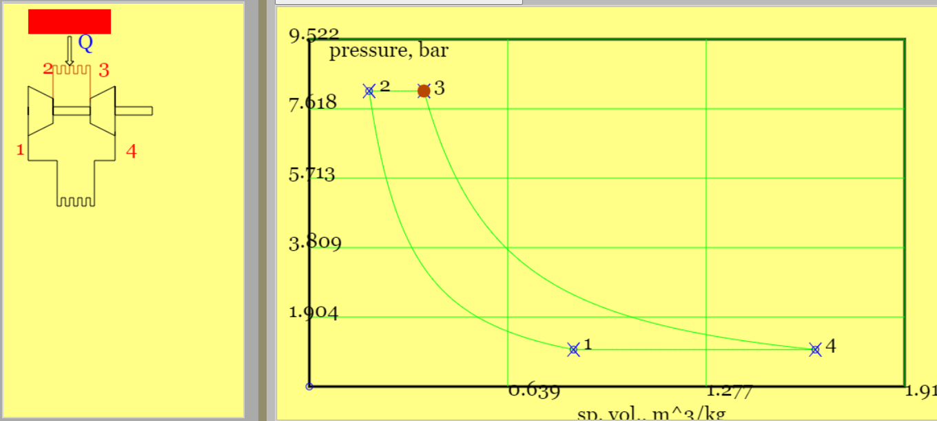
The classical theoretical Otto cycle is a simplified model of the petrol engine, developed by Nicholaus Otto. A pleasing outcome is a simple equation demonstrating that higher compression ratios increase cycle efficiency. A set of rather complicated physical phenomenae are idealised as the four thermodynamic processes on the pressure-versus-volume plot in Figure 2.
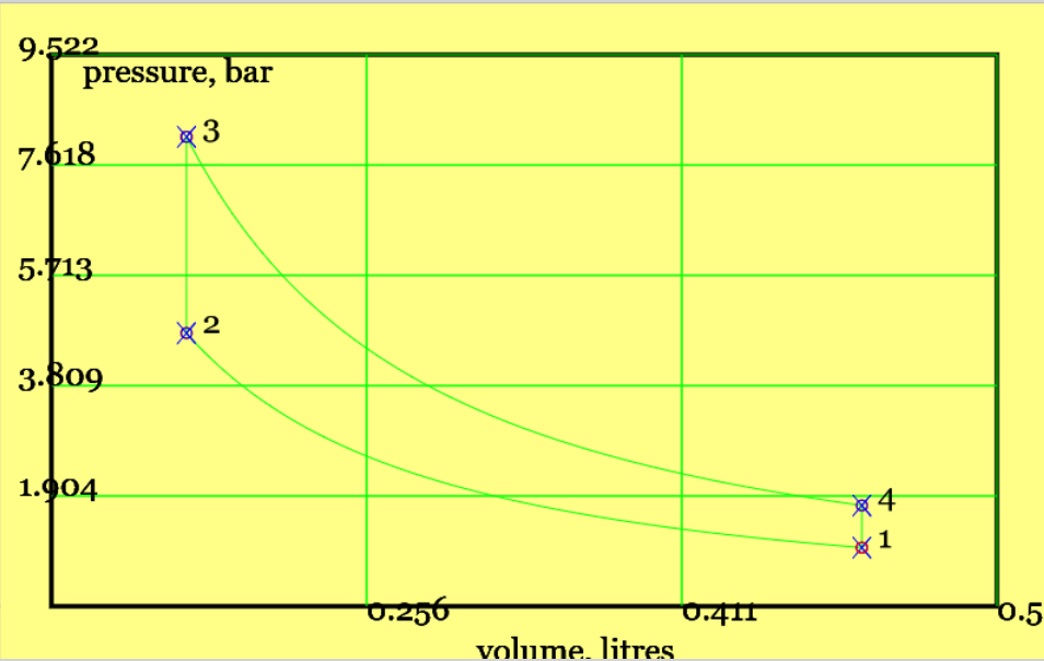
Figure 2. The theoretical Otto cycle (see linked animation of the cycle )
An animation of the cycle shows (theoretical) piston movement and process diagram (remember to press the "Otto Cycle" radio button). The four processes - two isentropic and two isochoric (constant volume) - are listed below.
Isentropic compression (1-to-2): the piston moves from BDC to TDC, compressing gas and increasing its pressure and temperature. There is no heat transfer. This is not too dissimilar to the compression stroke in the real world, although the latter is probably best described as "polytropic". The end temperature follows from the isentropic relationship, viz $$ T_2 = T_1 (\frac{V_1}{V_2})^{\gamma-1} = T_1 r_v^{\gamma-1} \qquad const. \; entropy $$
where \(r_v\) is the compression ratio defined earlier, a ratio of swept volumes at TDC and BDC.
Constant volume heat addition (2-to-3): the piston remains at TDC and heat is added with gas at constant volume. No work is done. The addition of heat from the hot reservoir to the cycle is, $$ |Q_H| \equiv |Q_{23}| = m c_v (T_3-T_2) \qquad const. \; volume $$
(In the real world, a spark would ignite typically 30 degrees of crank angle before TDC and, rather than occuring instantaneously, combustion would persist through much of the power stroke from TDC to BDC.)
Isentropic expansion (3-to-4): the piston moves from TDC to BDC, the gas decreases pressure and temperature and with no heat transfer. The end temperature follows from the isentropic relationship, viz $$ T_4 = T_3 (\frac{V_3}{V_4})^{\gamma-1} = T_3/ r_v^{\gamma-1} \qquad const. \; entropy$$
Constant volume heat rejection (4-to-1): the piston remains at BDC and the gas maintains a constant volume as it rejects heat to the cold reservoir. No work is done. The cyclic heat rejection is, $$ |Q_L| \equiv |Q_{41}| = m c_v (T_4-T_1) \qquad const. \; volume$$
In the real world, the equivalent heat rejection features an exhaust stroke (BDC to TDC) and an intake stroke (TDC to BDC). The first ejects hot, waste gases from the cylinder and the second takes in a cooler mixture of fuel vapour and clean air. The associated frictional resistance to gas flow reduces appreciably the engine's brake power.
The main feature of classical analysis is the estimation of cycle efficiency. In terms of the end-point temperatures, $$ \eta_{cyc} = 1- \frac{|Q_L|}{|Q_H|} = 1- \frac{T_4-T_1}{T_3-T_2} $$
One notes that the start and end temperatures of the two isentropic processes are both related by \( r_v ^{\gamma-1} \), $$ \frac{T_2}{T_1} = \frac{T_3}{T_4} = r_v^{\gamma-1} $$ Combination of the above two equations gives the well known result,
$$ \eta_{cyc} = 1-\frac{1}{r_v^{\gamma-1} } $$
Real-world cycle efficiencies are substantially less than calculated above. A more realistic model might allow for polytropic compression and expansion and gas friction losses associated with intake and exhaust. (Polytropic processes would create additional heat transfers to the cylinder.) This would give a more reasonable "indicated work" (net boundary work). But to get the "brake work" one must account further for the sliding friction of the piston inside the cylinder, and for friction losses in the power train.
Example 6.010: Reproduce the default results for our online simulator . A simple Otto cycle operates with a compression ratio of 4.5 (very low, and chosen for visual effect) , a (very high) inlet temperature of 500K, normal atmospheric pressure at inlet, a total cylinder volume of 0.5 litres at BDC, and a maximum temperature of \(T_3=1470 K \) after heat addition. Estimate the two remaining end-point temperatures, the energy transfers for each process, and cycle efficiency.
Solution: This problem concerns the performance of a simple Otto Cycle. Figure 2 Provides a pV diagram and the Ts diagram is available on the simulator (temperatures and compression ratios were chosen to make the separate processes stand out. (Use the simulator to experiment with real world values - e.g. standard temperature and a typical compression ratio might be 11.3.) The standard air cycle assumptions are made. Physical Laws include the Ideal Gas Law (to get the mass of gas), First Law (in the form of the Non-Flow Energy Balance), and isentropic relations.
The mass of material follows from the Ideal Gas Law. Note that the properties of dry air are used. I shall put conversion factors, ([atm to kN/m2] and [litres to m3]), in square brackets.
$$ m = \frac{p V_1}{R T_1} = \frac {1.013 \times [100] \times 0.5 \times [0.001]}{0.287 \times 500} = 0.353 \times 10^{-3} kg $$Use the isentropic relationship to obtain \( T_2 \)
$$ T_2 = T_1 (\frac{V_1}{V_2})^{\gamma-1} = T_1 r_v ^{\gamma-1} = 500 \times 4.5^{0.4} = 913 K$$ $$ U_2-U_1 = m c_v (T_2 - T_1) = 0.353 \times 10^{-3} \times 0.718 \times (913-500) = 105 \times 10^{-3} kJ $$For an isentropic compression there is no heat transfer and all internal energy is converted to work. To emphasise this argument, I use the Non Flow Energy Equation
$$ U_2-U_1 = Q_{12}+W_{12} \; ; \qquad Q_{12}=0 \implies W_{12}=U_2-U_1 = 0.105 kJ $$Because the heat addition process is at constant volume no work is done, and change in internal energy becomes heat addition.
$$ T_3 = 1470 K \qquad (given) $$ $$ U_3-U_2 = m c_v (T_3 - T_2) = 0.353 \times 10^{-3} \times 0.718 \times (1470-913) = 0.141kJ $$ $$ W_{23} =0 \implies Q_{23} = U_3-U_2 = 0.141 kJ $$Very similar ideas apply to the processes of isentropic expansion ...
$$ T_4 = T_3 / r_v ^{\gamma-1} = 1470 / 4.5^{0.4} = 805 K $$ $$ W_{34} = m c_v (T_4 - T_3) = -0.168 kJ \qquad (Q_{34}=0) $$... and constant volume heat rejection,
$$ Q_{41} = m c_v (T_1 - T_4) = -0.077 \times 10^{-3}kJ \qquad (Q_{34}=0) $$The net work input per cycle (compression + expansion) is,
$$W_{net} = W_{12} + W_{34} = -0.063 kJ $$and this should be equal and opposite to the net heat input. The cycle efficiency is the net work output per unit of heat input.
$$\eta_{cyc} = \frac{|W_{net}|}{Q_{23}} = \frac{0.063}{0.141} = 44.7 \% $$To check this I use the derived formula,
$$ \eta_{cyc} = 1-\frac{1}{r_v^{\gamma-1} } = 1-\frac{1}{4.5^{0.4}} = 45.2\% \qquad (OK,\; within \; rounding \;error) $$These three sets of results conform to the website simulation, so long as specifc heat input rather than \(T_3\) is used as an input (\(q_{23}=0.141 kJ/0.353 \times 10^{-3} kg = 400kJ/kg \) ).
For discussion - explain what happens to cycle efficiency when heat input is increased.
Tough exam setters may well specify polytropic compression. Bear in mind that both heat transfer and work transfer are then present and you must account for two heat inputs.
In the simplest theoretical Diesel cycle heat is added isobarically, with gas at constant pressure. The other processes match those in the theoretical Otto Cycle.
The cycle is rather similar to the Section 3's Otto cycle. The essential difference is that heat addition is at constant pressure. This constant pressure heating attempts to represent the observed real world direct injection of fuel into the cylinder. Injection starts at TDC, where temperatures are hot enough to ignite the fuel. (No spark is generated). The injection and the associated combustion continues for a finite movement of the piston. Injection is then "cut-off" and the piston continues its travel to BDC (and isentropically in the theoretical process).
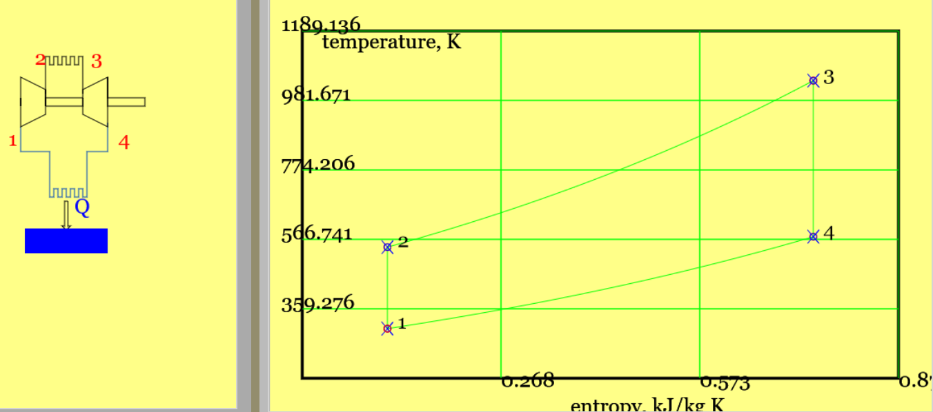
Figure 3 shows the cycle, comprising isentropic compression, isobaric heat addition, isentropic expansion and isochoric (constant volume) heat rejection.
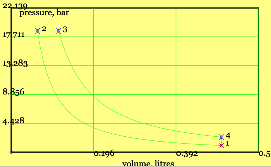
Figure 3. A Theoretical Diesel cycle (see linked animation of the cycle )
An animation of the cycle shows (theoretical) piston movement and process diagram (remember to press the "Diesel Cycle" radio button). The four processes are listed below. (Only one - constant pressure heat addition - differs from the theoretical Otto cycle.)
Isentropic compression (1-to-2): the piston moves from BDC to TDC, compressing gas and increasing its pressure and temperature. There is no heat transfer. The end temperature follows from the isentropic relationship, viz $$ T_2 = T_1 r_v^{\gamma-1}$$
Constant pressure heat addition (2-to-3): the piston moves from TDC to a position (marked as point 3 on the pV diagram) part way between TDC and BDC. The heat addition is, $$ |Q_H| \equiv |Q_{23}| = m c_p (T_3-T_2) $$
Because pressure is maintained constant, the start and end temperatures are related by the cut-off ratio. This is the gas volume when the fuel supply is "cut-off", divided by the volume with the piston at TDC. $$ T_3 = \frac{V_3}{V_2} T_2 = r_{cut}T_2 $$
In modern engines, there would be three or four successive, sharp pulses of fuel injection, rather than a steady flow, designed so as to reduce the formation of nitrous oxides. (Thus more complicated models might idealise injection as successive isobaric and isochoric processes.)
Isentropic expansion (3-to-4): the piston to TDC, decreasing pressure and temperature. The end temperature follows from the isentropic relationship. To get \(T_4\) we need the ratio of volume at BDC to volume at cut-off. $$ \frac{V_4}{V_3} = \frac{V_1}{V_3} = \frac{V_1}{V_2} \frac{V_2}{V_3} =\frac{r_v}{r_{cut}} $$ Thereupon, $$ T_4 = T_3 (\frac{V_3}{V_4})^{\gamma-1} = T_3 (\frac{r_{cut}}{r_v})^{\gamma-1}$$
Constant volume heat rejection (4-to-1): the piston remains at BDC and heat is rejected at constant volume. The heat rejection is, $$ |Q_L| \equiv |Q_{41}| = m c_v (T_4-T_1) $$
An important feature of classical analysis is the estimation of cycle efficiency. Remember that different types of heat capacity are employed to obtain \( Q_L \) and \(Q_H\). In terms of the end-point temperatures, $$ \eta_{cyc} = 1- \frac{|Q_L|}{|Q_H|} = 1- \frac{1}{\gamma} \frac{T_4-T_1}{T_3-T_2} $$
This is also written in terms of the cut-off and compression ratios. One algebra trick is to write all other temperatures in terms of \(T_1\). $$ T_2 = r_v^{\gamma-1} T_1 \qquad const. \; entropy $$ $$ T_3 = r_{cut}T_2 = r_{cut} r_v^{\gamma-1} T_1 \qquad const. \; pressure$$ $$ T_4 = (\frac{r_{cut}}{r_v})^{\gamma-1} T_3 = r_{cut}^{\gamma} T_1 \qquad const. \; entropy $$
Substitute the above into the expression for \( \eta_{cyc} \) to get,
$$ \eta_{cyc} = 1 - \frac{1}{\gamma r_v^{\gamma-1}} \frac{r_{cut}^{\gamma}-1}{r_{cut}-1} $$
Example 6.020: Reproduce the default results for our online simulator . A simple Diesel cycle operates with a compression ratio of 8 (very low, and chosen for visual effect) , a (very high) inlet temperature of 500K, normal atmospheric pressure at inlet, a total cylinder volume of 0.5 litres at BDC, and a cut-off ratio of 1.8. Estimate the end-point temperatures, the energy transfers for each process, and cycle efficiency.
Solution: This problem concerns the performance of a simple Diesel Cycle. Figure 3 provides a pV diagram and the Ts diagram is available on the simulator. (Temperatures and compression ratios were chosen to make the separate processes stand out.) Physical Laws are listed in Example 6.010.
The mass of material was calculated in example 6.010 by the Ideal Gas law. The temperature after compression follows an isentropic relationship (there is a new compression ratio ) and use the heat capacity to get \(W = \Delta U \)
$$ m = 0.353 \times 10^{-3} kg \qquad (previous) $$ $$ T_2 = 500 \times 8^{0.4} = 1149 K$$ $$ W_{12} = U_2-U_1 = m c_v (T_2 - T_1) = 0.164 kJ \qquad (Q_{12}=0) $$During heat addition pressure is taken as constant and the Ideal Gas Law reduces to Charles' Law, \(T \propto V \).
$$ T_3 = r_{cut} \times T_2 = 1.8 \times 1149 = 2068 K $$During the constant pressure expansion heat transfer and work transfer are both at play. Here, I shall explore a few, consistent methods of finding these. Firstly, work, formally defined as force times distance, is equal to the multiple of the constant pressure and volume change,
$$ W_{23} = -p' (V_3 - V_2) \qquad where \; p'=p_2=p_3 $$To get the three components above,
$$ V_2 = V_1 / r_v = 0.5/8 = 0.0625 litres \; ; \qquad p_2 = (\frac{V_1}{V_2})^{\gamma-1} p_1 = r_v^{1.4} p_1 = 18.6 bar; \qquad v_3 = r_{cut} V_2 = 1.8 \times 0.0625 = 0.1125 litres $$ $$ W_{23} = -p' (V_3 - V_2) = -18.6 \times [100] \times (0.1125-0.0625) \times [0.001] = -0.093 kJ $$where the square brackets, [], contain unit conversion factors. Alternatively p and V can remain unknown but manipulated with the Ideal Gas Law.
$$ W_{23} = -p_3 V_3 + p_2 V_2 = -m R(T_3-T_2) = -0.353 \times 10^{-3} \times 0.287 \times (2068-1149) = -0.093 kJ \qquad (OK) $$Two, consistent alternative calculations are available for heat transfer. Noting that at constant pressure enthalpy change is equal to heat input, one can simply apply the isobaric heat capacity thus,
$$ Q_{23} = m c_p (T_3-T_2) = 0.353 \times 10^{-3} \times 1.005 \times (2068-1149) = 0.326 kJ $$Or we can can find the change in internal energy and then apply the Non Flow Energy Equation.
$$ U_3-U_2 = m c_v (T_3-T_2) = 0.353 \times 10^{-3} \times 0.718 \times (2068-1149) = 0.232 kJ $$ $$ Q_{23}= U_3-U_2 - W_{23} = 0.232 - (-0.093) = 0.326 kJ \qquad (OK) $$
The remaining expansion from 3 to 4 is isentropic, with volume ratio \( V_4/V_3 = r_v / r_{cut} = 8/1.8 \). The end temperature is and work are
. $$ T_4 = \frac{2068 }{(8/1.8)^{0.4}} = 1139 K $$ $$ W_{34} = m c_v (T_4-T_3) = 0.353 \times 10^{-3} \times 0.718 \times (1139-2068) = - 0.235 kJ \; ; \qquad Q_{34}=0 $$For the final, heat rejection stage,
$$ Q_{41} = U_1-U_4 = m c_v (T_1-T_4) = 0.353 \times 10^{-3} \times 0.718 \times (500-1139) = -0.162kJ \; ; \qquad W_{41}=0 $$So the net work per cycle is
$$ W_{net} = W_{12}+W_{23}+W_{34} + W_{41} = 0.164 - 0.093 -0.235+0 = -0.164kJ $$The cycle efficiency is net work per unit heat input.
$$ \eta_{cyc} = \frac{Q_{23}}{|W_{net}|} = \frac{0.164}{0.326} = 50.3 \% $$Check this by using the derived formula.
$$ \eta_{cyc} = 1 - \frac{1}{\gamma r_v^{\gamma-1}} \frac{r_{cut}^{\gamma}-1}{r_{cut}-1} $$ $$ \eta_{cyc} = 1 - \frac{1}{1.4 \times 8^{0.4}} \frac{1.8^{1.4}-1}{1.8-1} = 1 - 0.564 \times 1.596 = 50.4\% \qquad (OK) $$The computed energy flows conform to the web-based calculation.
The theoretical Stirling cycle comprises two reversible isothermal processes and two reversible constant volume processes with internal gas-to-regenerator-to-gas heat transfer.
The Stirling cycle is driven by external heating. The working fluid - possibly air - is sealed within the engine. In the theoretical model the exchanges of heat with two external heat reservoirs determine uniquely the cycle efficiency. A "regenerator" - a set of "mini reservoirs" inside the engine boundary - beneficially recovers heat from a constant volume cooling process and transfers it to a constant volume heating process. The three common types of practical cycle are termed "alpha", "beta", and "gamma" types. The animated engines website offers a good explanation of the mechanical operation of the alpha type engine and the role of its regenerator .
In theoretical analysis, it is common practice to show the cycle as a T-s diagram, Figure 4. The four processes are listed below the figure.
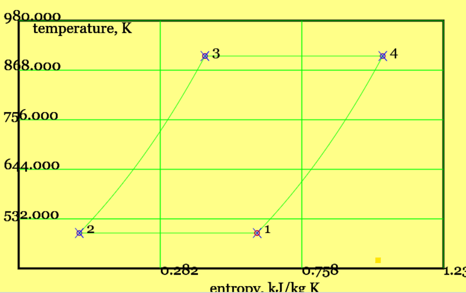
Figure 4. The Stirling cycle, shown as a Ts diagram (see linked animation of the cycle )
Isothermal cooling and contraction (1-to-2): the gas temperature is constant, and heat transfer is reversible case when only an infinitessimal temperature driving force applies. Then the cold reservoir temperature follows \(T_2 = T_1 \equiv T_L\). For an isothermal process with ideal gas there is no change in internal energy and the moving boundary work is equal and opposite to heat addition. We shall see that there is no great need of algebraic manipulation to obtain cycle efficiency, \(\eta_{cyc}=1-T_L/T_H\). Nonetheless, it is instructive to define the heat rejection, $$ |Q_L|\equiv |Q_{12}| = |W_{12}| = mRT_L ln (\frac{V_1}{V_2}) = mRT_L \, ln (r_v) $$ where \(r_v\) is the compression ratio, applying from BDC to TDC
Internal heating at constant volume (2-to-3): this raises the working gas temperature from \(T_L\) to \(T_H\). The gas accepts heat from a regenerator , which I like to imagine as a long series of "mini reservoirs" at temperatures \( T_L, T_L +1, T_L +2 ... T_H \). Each part of the heat transfer is from a mini-reservoir at (very nearly) the same temperature as the working gas; the heat transfer is thus reversible. The total internal heat transfer is, $$ |Q_{int,23}| = m c_v (T_3-T_2) = m c_v (T_H-T_L) $$
Isothermal heating and expansion (1-to-2): again, temperature is constant and to maintain reversibility the temperature driving force is infinitessimally small. Hence \(T_4 = T_3 = T_H\). The heat addition, is $$ |Q_H|= |W_{34}| = mR T_H \; ln (r_v) $$
Internal cooling at constant volume (4-to-1): the working gas now rejects heat to the regenerator, in the reverse of constant volume heat addition, 2-3. The amounts of internal heat addition and rejection are equal, viz, $$ |Q_{int,41}| = m c_v (T_4-T_1) = m c_v (T_H-T_L) = |Q_{int,23}| $$
Evaluating the cycle efficiency of a reversible machine is very easy. From the third corollary of the Second Law of Thermodynamics , for given \(T_L, T_H \) the cycle efficiency is the same for any reversible machine. The Carnot Efficiency holds true,
$$\eta_{cyc} = 1 - \frac{T_L}{T_H} $$
A useful exercise is to obtain this result by substituting the above estimates of \(Q_L, Q_H\) into the efficiency equation. In my own humble opinion this serves as a sanity check rather than a rigorous proof.
Real world machines exhibit several imperfections. No regenerator is perfectly effective, and an inability to transfer all required heat between the two constant volume processes leads to greater demand on external heating and cooling. External heat transfers in themselves demand substantial temperature differences between the reservoirs and working gas, leading to irreversiblilities (see Figure 7 in the linked webpage). In the real machines the connection of the two pistons to the same crankshaft renders imperfect the assumptions of isochoric and isothermal processes. In this particular regard the Schmidt cycle offers a better model.
Schmidt analysis offers improved analysis of the Stirling Engine. I shall develop this section eventually, but in the meantime some good notes are produced by Prof Khirata
Consider an animation of a alpha-type Stirling engine . You will observe two cylinders: in the simplest analysis the "hot cylinder" is assumed to hold gas at reservoir temperature \(T_H\) and the "cold cylinder" is assumed to hold gas at reservoir temperature \(T_L\). The crankshaft and connecting rods do not allow for constant volume heating/ cooling stages. You will notice, on Prof Khirata's web page, that the pV diagram shows a continuous loop, rather than four distinct processes.
The steady-flow, closed Brayton Cycle comprises two isentropic processes and two isobaric processes.
Variants of the Brayton cycle are used for power generation and marine propulsion. In the basic real-world plant (1) air is compressed in steady flow (2) fuel is added to the air and the mixture ignited in a combustion chamber (3) the exhaust gases, at elevated temperature and pressure, drive a turbine in steady-flow. The turbine is "bootstrapped" to the compressor via a common shaft; some of the turbine's power output drives the compressor. The remaining shaft power is employed in propulsion or to generate electricity. The air-to-fuel ratio is very high, typically 50: 1, and so in the theoretical cycle one might well employ with modest accuracy the thermodynamic properties of air.
In the equivalent air standard cycle, a heat input replaces the combustion chamber, and a fictitious heat output closes the cycle. (In reality, cooling the turbine exhaust and returning it to the compressor would fail because no oxygen would remain to support combustion.) Let us start with a version of the cycle wherein all processes are reversible. The engine will admit air at atmospheric pressure and temperature, compress the air so that the pressure increases \( r_p \) times, heat the air, and expand it back to one atmosphere pressure. Plant and process diagrams follow.
(a) (b)
Figure 5. The basic Brayton cycle, shown with (a) highlighted heat addition and a pV diagram,(b) highlighted heat rejection and a Ts diagram. (See linked animation of the cycle. )
From the p-V diagram, compression and expansion are essential to ensure the net reversible work (the area of shape 1-2-3-4-1) exceeds zero. One neglects pressure changes within the combustor (2-3) or (ficticious) heat rejection (4-1). Both intake (1) and exhaust (4) are taken as being at the pressure of the surroundings. Heat transfers follow from the Steady Flow Energy Equation. I shall here ignore kinetic energy and potential energyy changes. In the following it is useful to note that heat input is in proportion to \(T_3 - T_2\).
Heat addition and heat rejection (ignore changes in potential and kinetic energy, any frictional heating)
$$ \dot{Q}_{in} = \dot{m} (h_3-h_2) = \dot{m} c_p (T_3-T_2) $$ $$ \dot{Q}_{out} = \dot{m} (h_1-h_4) = \dot{m} c_p (T_1-T_4) $$Where \( \dot{Q}_{in} \) and \( \dot{Q}_{out} \) refer respectively to heating power input and heating power output (or loss). Provided that changes in kinetic and potential energy are unimportant the heating powers yield ...
Cycle efficiency
$$ \eta_{cyc} = 1 - \frac{|\dot{Q}_{out}|}{|\dot{Q}_{in}|} = 1 - \frac{T_4-T_1}{T_3-T_2} $$Piston-cylinder engines are naturally specified with a ratio of volumes (the compression ratio); open cycles with steady flow are naturally specified with a ratio of pressures. Thus compressor inlet and outlet temperatures are related by the isentropic relationships
$$ T_2 = T_1 \; \frac{p_2}{p_1}^{(\gamma-1)/\gamma} = T_1 \; r_p^{(\gamma-1)/\gamma} $$where \(r_p = p_2/p_1 \) is the pressure ratio. (For some students the exponent \( (\gamma-1)/\gamma\) will look intimidating. For air, \(\gamma=1.4\), its replacement with \(\frac{2}{7}\) may well offer a friendlier approach.) The same pressure ratio applies to the turbine inlet and outlet temperatures follow,
$$ T_4 = T_3 \; \frac{p_4}{p_3}^{(\gamma-1)/\gamma} = T_3 \;/ r_p^{2/7} $$The isentropic relationships can be used to replace the denominator term in cycle efficiency, viz. \(T_3=T_4 r_p^{(\gamma-1)/\gamma} \) and \( T_2 = T_1 r_p^{(\gamma-1)/\gamma} \)
$$ \eta_{cyc} = 1 - \frac{1}{ r_p^{(\gamma-1)/\gamma} } $$The SFEE yields the net work output. Some turbine work is used to drive the compressor; the net work output is the difference between the two.
$$ \dot{W}_{12} = \dot{m} c_p (T_2-T_1) \qquad compressor $$ $$ \dot{W}_{34} = \dot{m} c_p (T_4-T_3) \qquad turbine $$ $$ \dot{W}_{net} = \dot{W}_{12} + \dot{W}_{34} = \dot{m} c_p (T_2-T_1+T_4-T_3) \qquad net \; useful \; output $$Real world compressors and turbines never work isentropically - the isentropic efficiency defined in Topic 4 pertains. Also friction losses apply in the combustion chamber / heater - the outcome can be shown on process diagrams. Please see notes concerning the isentropic efficiency of turbines and the isentropic efficiency of compressors . A worked example serves to illustrate the calculation procedure.
Example 6.030: A simple Brayton cycle operates with a pressure ratio of 9.5, a temperature at compessor inlet of 300K and a temperature at turbine inlet of 1250K. Estimate all specific work transfers, all specific heat transfers and the cycle efficiency. Take the compressor and turbine as operating (a) both reversibly (b) with respective isentropic efficiencies of 85% and 90%
Solution: This problem concerns the performance of a simple Brayton Cycle. Suitable plant and process (pV) diagrams are provided above or can be generated with the simulation on our website. The standard air cycle assumptions are made; in particular the thermophysical properties of air as an ideal gas are employed and one notes a constant isobaric heat capacity. The bootstrap, connecting compressor and turbine, is treated as working perfectly, with mechanical efficiency of 100%. The plant inlet and exit pressures are treated as identical. The analysis is for steady operation and excludes start up and shut down aspects. The relevant physical principles are the Ideal Gas Law that relates pressure, temperature and volume with simple equations, the Steady Flow Energy Equation (a corrolary of the First Law) and the isentropic relationships (derived from the NFEE, IGL and work definition). It is useful to note that \(c_p=1.005\) and \( (\gamma-1)/\gamma = 2/7 \).
Starting with the reversible compression and expansion, use the isentropic relationship to get unknown temperatures.
$$ T_2 = T_1 r_p^{2/7} = 300 \times 9.5^{2/7} = 571 K $$ $$ T_4 = T_3/r_p^{2/7} = 1250/9.5^{2/7} = 657 K $$The specific transfers of energy are then,
$$ w_{12} =h_2-h_1 = c_p (T_2-T_1) = 1.005 \times (571-300) = 272 kJ/kg \qquad (compressor) $$ $$ q_{23} = h_3-h_2 = c_p(T_3-T_2) = 1.005 \times (1250-571) = 682 kJ/kg \qquad (heat \; addition) $$ $$ w_{34} = h_4-h_3 = c_p (T_4-T_3) =1.005 \times ( 657 - 1250) = -596 kJ/kg \qquad (turbine) $$ $$ q_{41} = h_1-h_4 = c_p (T_1-T_4) = 1.005 \times (300-657) = -359 kJ/kg \qquad (ficticious \; loss)$$The net power production and efficiency are,
$$ w_{net}=w_{12}+w_{34}=-324 kJ/kg $$ $$ \eta_{cyc} = \frac{|w_{net}|}{q_{23}}= \frac {324}{682}=47.5\% $$Check
$$ \eta_{cyc}=1-\frac{1}{r_p^{2/7}} = 1-1/9.5^{2/7} = 47.4 \% \qquad (OK) $$(The two estimates are identical, within rounding error.) Let us consider the anisentropic compression and expansion .
$$ w_{12}= w_{12,isen}/ \eta_{isen} = 272/0.85 = 320 kJ/kg $$ $$ w_{34} = w_{3,isen}/\eta_{isen} = 0.9 \times (-596) = -536 kJ/kg $$The SFEE yields the temperature at the compressor exit.
$$ w_{12}=c_p (T_2-T_1) \implies T_2=T_1-w_{12}/c_p = 618K$$Alternatively, provided that gas is ideal so that specific enthalpy is proportional to temperature,
$$ (T_2-T_1)=(T_{2,isen}-T_1)/\eta_{isen} \implies T_2=T_1(1-1/\eta_{isen}) +T_{2,isen}/\eta_{isen} = 619K \qquad (OK)$$The modified specific input of heat is,
$$ q_{23} = c_p (T_3-T_2) = 1.005 \times (1250-618) = 635 kJ/kg $$And the cycle efficiency is reduced to,
$$ \eta_{cyc} = \frac{|w_{12}+w_{34}|}{q_{23}} = \frac{| 320-536 | } {635 } = 34.0 \% $$These two sets of results conform to the website simulation, so long as heat input rather than \(T_3\) is used as an input.
A regenerator usefully recovers heat within the boundary of the plant and thereby reduces the demand for external heat .
More sophisticated plant can improve cycle efficiency or power output. Provided that the turbine exhaust is hotter than the compressor exhaust, some thermal energy can be recovered usefully from the turbine exhaust before said thermal energy is rejected to the surroundings. This internal heat transfer is achieved by a heat exchanger known as a "regenerator" or a "recuperator".
The purpose of a heat exchanger is to transfer heat from one stream of fluid to another, without allowing the two streams to mix. Examples of heat exchangers include automobile radiators and the internal fire tubes of locomotive boilers. In an abstract form, one might imagine the heat transfer surface as a horizontal flat plate, with hot fluid flowing above the plate and colder fluid below; heat passes from the hot fluid through the plate to the colder fluid. The recuperator is shown between points 2, 3, 5 and 6 on Figure 6. Energy recovered from the turbine exhaust (at 5) is transferred as heat to the colder compressed air (initially at 2), before heat addition from an external hot reservoir at locations 3-4.
(a) (b)
Figure 6. The Brayton cycle with regenerator (100% effectiveness) (a) highlighted primary heat addition and a pV diagram,(b) highlighted heat recovery (in the regenerator) and a Ts diagram. The regenerator is potentially useful if \(T_5 > T_2\). (See linked animation of the cycle. )
The Clausius Statement of the Second Law tells us that \( T_3 \leq T_5 \). Therefore the maximum temperature achievable in the regerator exit, and the associated maximum heat recovery, are
$$ T_{3,max} = T_5 $$ $$ \dot{Q}_{23,max} = \dot{m} c_p (T_{3,max}-T_2) = \dot{m} c_p (T_5-T_2) $$The exchanger performance can be defined by by "effectiveness", \( \epsilon \) ,
$$ \epsilon = \frac {\dot{Q}_{23} } {\dot{Q}_{23,max} } $$Recall that the cycle efficiency concerns the net transfers of work and heat with the external surroundings of the plant. The internal heat transfer \( \dot{Q}_{23} \) - inside the boundary of the plant - is excluded the denominator of the fraction that is cycle efficiency .
$$ \eta_{cyc} = \frac{|\dot{W}_{net}|}{\dot{Q}_{in}} = \frac{\dot{m} c_p (T_5-T_4) + \dot{m} c_p (T_2-T_1)}{\dot{m} c_p (T_4-T_3)} = \frac{T_5-T_4+T_2-T_1}{T_4-T_3} $$Example 6.040: A Brayton cycle with recuperator operates with reversible compression and expansion. The air inlet temperature is \(T_1 = 300 K \) and the pressure ratio is 10. Estimate the cycle efficiency if the turbine inlet temperature is \(T_4=1350K\) and the recuperator effectiveness is (a) 0 %, (b)100% (c) 80%.
Solution: I shall use diagrams above. The assumptions and physical laws in the previous example are repeated. In addition we shall take an energy balance over the regenerator. Start by setting the (a) effectiveness to 0%.
$$ T_3 = T_2 = T_1 \times r_p ^{ 2/7} =300 \times 10^{2/7 } = 579 K \qquad compressor \; outlet$$ $$ T_6 = T_5 = 1350/10^{2/7} = 699 K \qquad turbine \; outlet$$Apply the SFEE to get the specific addition of heat.
$$ q_{34} = c_p (T_4-T_3) = 1.005 \times (1350-579) = 775 kJ/ kg \qquad specific \; input \; of \; heat $$The specific work output is the summation of signed compressor and turbine work.
$$ w_{net} = | w_{12}+w_{45} | = c_p |T_2-T_1+T_5-T_4| = 1.005 \times |579-300+699-1350| = 374 kJ/kg \qquad net \; specific \; work $$Use two methods to get cycle efficiency.
$$ \eta_{cyc} = \frac{w_{net}}{q_{34}} = 374/775 = 48.2\% $$or
$$ \eta_{cyc} = 1 -\frac{1}{r_p^{2/7}} = 1-\frac{1}{10^{2/7}} = 48.2 \% \qquad (OK) $$Now consider (b) a regenerator with 100% effectiveness . The heat exchanger brings the temperature of compressed air to that of the turbine exhaust, viz
$$ T_3 \equiv T_{3,max} = T_5 = 699 K $$The higher value of \(T_3\) reduces the demand for heating ( \(T_3\) was 579K ) so that,
$$ q_{34} = c_p (T_4-T_3) = 1.005 \times (1350-699) = 654 kJ/ kg $$The temperatures in-and-out of the compressor are unchanged, likewise the temperatures in-and-out of the turbine, so the net specific work output is unchanged. The efficiency is thus.
$$ \eta_{cyc} = \frac{w_{net}}{q_{34}} = 374/654 = 57.2\% $$Let us consider an alternative approach and find the recovered heat
$$ q_{23} \equiv q_{23,max} = c_p (T_3-T_2) = 1.005 \times (699-579) = 121 kJ/ kg $$This is subtracted from the externally transferred \(q_{34}\) with no heat recovery (part (a) above). The modified heat addition from the hot reservoir is,
$$ q_{34} = q_{34}^{NHR}-q_{23} = 775-121 = 654kJ/kg $$Where NHR indicates "no heat recovery", calculated in part (a) above. The improved cycle efficiency is,
$$ \eta_{cyc} = \frac{w_{net}}{q_{34}}= \frac{374}{654} =57.2\% \qquad (OK) $$Let us now consider operation (c) operation of the regenerator at 80% effectiveness. The recovered heat and primary heat transfer are,
$$ q_{23} = 0.8 \times q_{23,max} = 0.8 \times 121 = 97 kJ/ kg $$ $$ q_{34} = q_{34}^{NHR}-q_{23} = 775-97 = 678kJ/kg $$The cycle efficiency becomes,
$$ \eta_{cyc} = \frac{w_{net}}{q_{34}}= \frac{374}{678} =55.2\% $$These three sets of results conform to the website simulation, so long as heat input rather than \(T_4\) is used as an input.
Intercooling and reheating increase net specific work. Intercooling reduces the demand on compressors; reheating increases the output of turbines. The resulting increased external heat addition should be mitigated with a regenerator.
Previous notes introduced the concepts of intercooling for compression and reheating for expansion .
One option on this website's Brayton Cycle model features two compressors; the exhaust from compressor 1 is cooled to the initial inlet temperature. Likewise there are two turbines; the exhaust from turbine 1 is reheated to the original inlet temperature. Whereas reheating increases the specific power from the plant, a side effect is that exhaust gases are hotter. In practice, nearly all such plant is fitted with a regenerator (see above). For the sake of simplicity, the regenerator is omitted from the simulator and some discussion in this section.
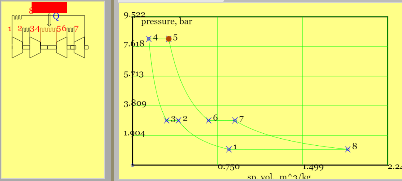
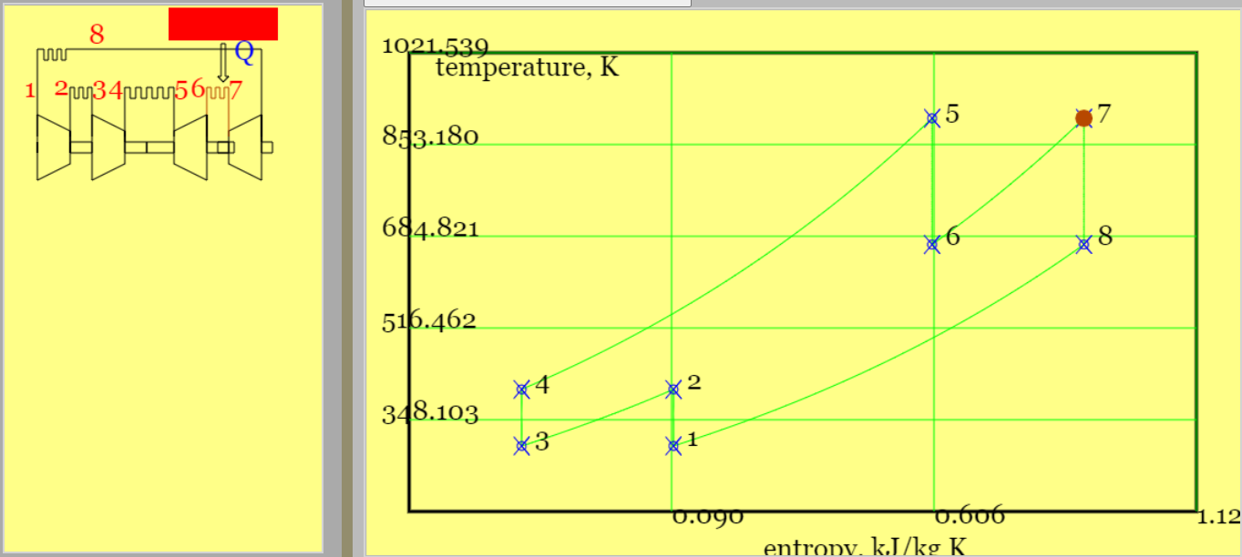
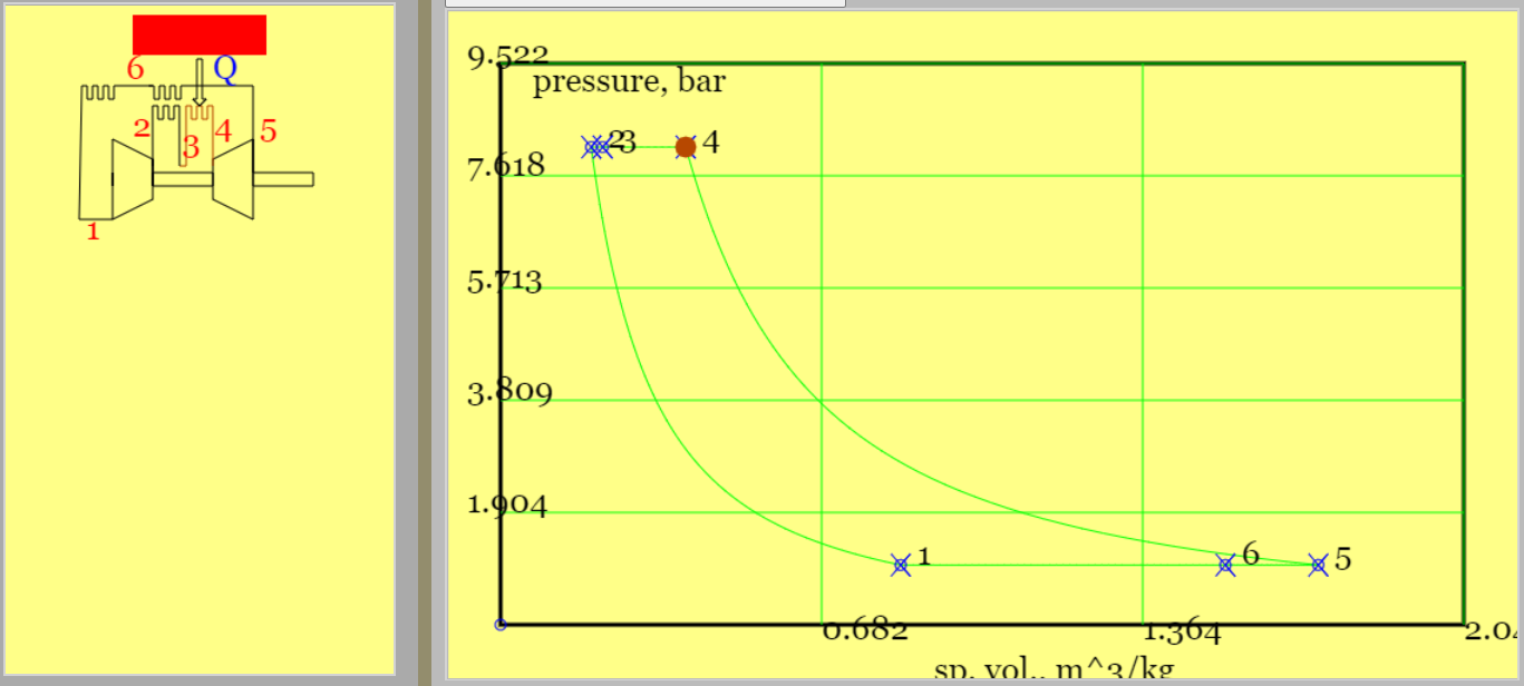
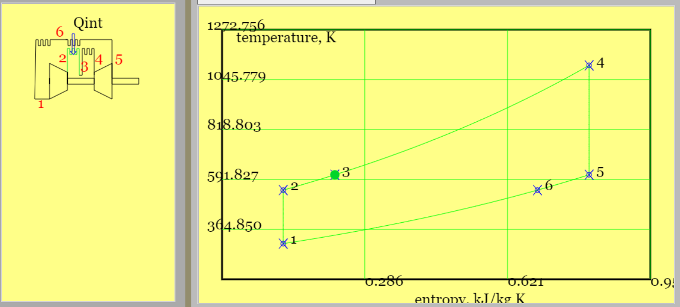
(a) (b)
Figure 7. The Brayton cycle with intercooling and reheat (regenerator omitted for sake of simplicity) (a) highlighted primary heat addition and a pV diagram,(b) highlighted reheat and a Ts diagram. That \( T_8 >> T_4 \) demonstrates the requirement for a regenerator.(See linked model of the cycle. )
;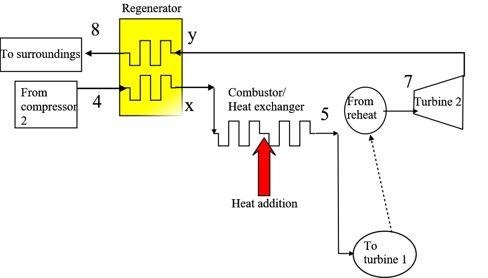
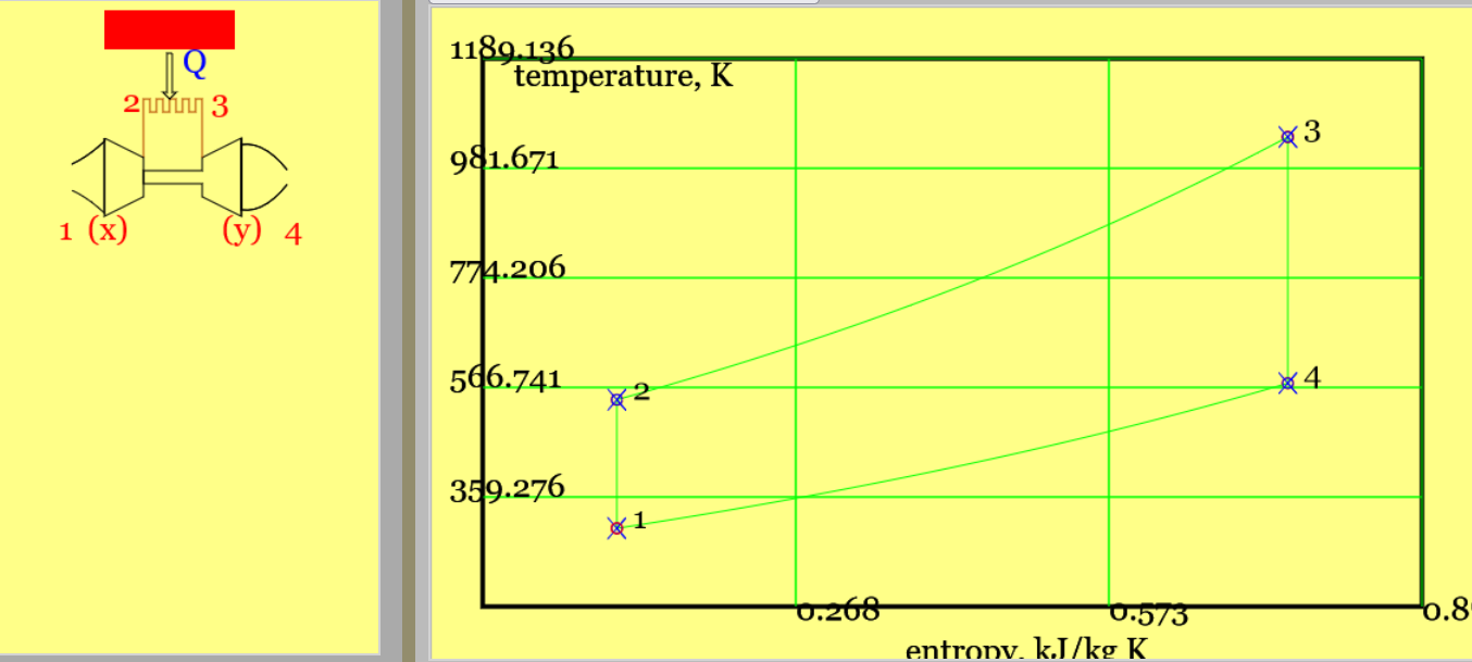
Figure 8. The layout for a regenerator, to be incorporated into the plant on Figure 7. Streams x and y are new streams.
For a given overall pressure ratio, \(r_{p,ov} \), the best pressure ratio for a single compressor or turbine is,
$$ r_{p,i} = \sqrt{r_{p,ov}} $$For example,
$$ \frac{p_2}{p_1} = \sqrt{\frac{p_4}{p_1}} $$In terms of the Second Law, in part 6-7 of the cycle reheat brings about heat addition to working fluid at a temperature closer to that of the hot reservoir, \(T_H\) and in part 2-3 intercooling brings about heat rejection from working fluid at a temperature closer to that of the cold reservoir , \(T_L\). Nonetheless, during the final heat rejection, part 8-1 (Figure 7), the comparatively high temperature of the turbine exhaust motivates the further addition of a regenerator (Figure 8).
Example 6.050: Run the Brayton Cycle model with intercooling and reheat. Note that for the default conditions \(q_{45} = 500 kj/kg \implies T_5=901 K\) and \(r_{p,ov}=8\). Compare the work of compression and expansion for this process with a simple Brayton cycle with the same pressure ratio. Estimate the maximum possible heat recovery and its impact on cycle efficiency.
Solution: The problem concerns the possible advantages of intercooling, reheat and regeneration. Assumptions and physical laws are similar to those used previously. For the intercooling and reheat note the further assumptions that \(T_3=T_1\) and \(T_7=T_5\) , and that compression and expansion are reversible/ isentropic.
First get the compressor and turbine exit temperatures.
$$T_4 = T_2 = T_1 \times r_{pi}^{2/7} = T_1 \times \sqrt{r_{p,ov}}^{2/7} = T_1 \times r_{p,ov}^{1/7} = 300 \times 8^{1/7} = 404K \qquad (compressors) $$ $$ T_8 = T_6 = T_5/ r_{p,ov}^{1/7} = 901/8^{1/7} = 669 K \qquad (turbines) $$Use SFEE to obtain total compressor work and total turbine work. The total gives the net work.
$$ w_{c,tot} = 2 c_p (T_2-T_1) = 2 \times 1.005 \times(404-300) = 209 kJ/kg $$ $$ w_{t,tot} = 2 c_p (T_6-T_5) = 2 \times 1.005 \times (669-901) = -466 kJ/kg $$ $$ w_{net} = 209-466 = -257 kJ/kg $$Compare against a simple Brayton cycle with single compressor and turbine. I used the online simulator with heat input reduced to 360 kJ/ kg to get the same maximum temperature of 901K and \(w_c = 245 kJ/kg \), \(w_t = 406 kJ/kg \), and \(w_{net}=-161 kJ/kg\). The simple cycle offers less net specific work for the same maximum temperature but for the time being note (i) the cycle efficiency of 45% (ii) given \(T_4 < T_2\) a regenerator would not benefit the simple cycle.
Confirm that the values of \(q_{45} \;and \; T_5 \) provided are consistent with SFEE.
$$ q_{45} = c_p (T_5-T_4) = 1.005 \times (901-404) = 499 kJ/kg \qquad (confirms \; heat \; input \; given) $$Work out the reheat, thereupon total heat input and cycle efficiency.
$$ q_{67} = c_p (T_7-T_6) = 1.005 \times (901-669)= 233 kJ/kg \qquad (reheat) $$ $$ q_{in} = q_{45} + q_{67} = 732 kJ/kg $$ $$ \eta_{cyc} = \frac{|w_{net}|}{q_{in}}= \frac{257}{732} = 35.1\% $$For purposes of comparison, the efficiency of the simple Brayton cycle is,
$$ \eta_{cyc,simple} = 1 - \frac{1}{r_{p,ov}^{2/7}} = 1-\frac{1}{8^{2/7}} = 44.8\%$$A cycle efficiency less than that of the simple Brayton cycle emphasises the requirement for a regenerator. Furthermore the Ts diagram on Figure 7 highlights the appreciable difference in temperature between \(T_8\) (turbine exhaust) and \(T_4\) (compressor outlet). Figure 8 above shows new streams, labelled x and y, that accommodate an additional heat exchanger. (Stream x is HX cold stream outlet and y is HX hot stream outlet.)
The maximum heat is recovered when \(T_{x,max}= T_8 \),
$$ q_{rec,max} = c_p (T_{x,max}-T_4)= c_p (T_8-T_4) = 1.005 \times (669-404) = 266kJ/kg $$This is subtracted from the original heat input so that the best cycle efficiency would be.
$$ \eta_{cyc} = \frac{257}{732-266} = 55.2\% \qquad (regenerator \; 100\% \; effective )$$Rather than generating power, the purpose of a turbojet cycle is to accelerate fluid and thereby generate thrust.
Wikipedia offers a good diagram of the turbojet engine. Figures 9 presents an abstract version, with process diagrams.
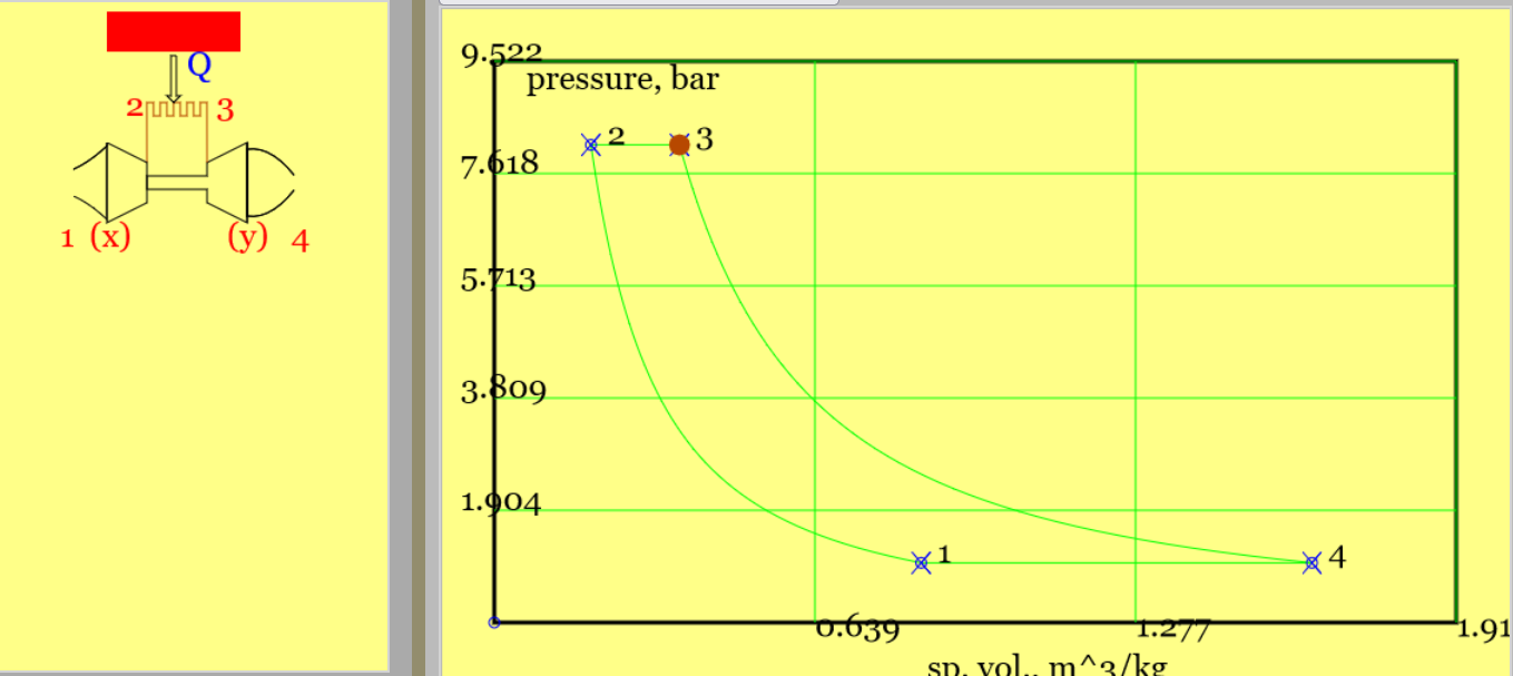
(a) (b)
Figure 9. A simplified turbojet cycle (only isentropic processes of compression and expansion are considered) with 1-x intake, x-2 compressor, 2-3 heat addition, 3-y turbine, y-4 nozzle. (a) a pV diagram, showing heat addition(b) a Ts diagram. (See linked model of the cycle. )
This cycle resembles the Brayton cycle. The principle purpose is to produce thrust rather than a net amount of power; the only power produced is that demanded by the turbine. The overall effect of the cycle is to convert the addition of heat to an increased kinetic energy of air passing through the engine; this means an increase in velocity, an increase in gas momentum and hence a thrust. Note that the air frame is travelling at speed \(v_1\) so that on a calm day an observer in the cockpit will "see" packets of air approach the engine at speed \(v_1\); this is the relative velocity of the air, in the frame of reference of the airframe or engine. In our analysis we shall employ most of the standard air cycle assumptions. However, changes in kinetic energy are considered between 1-and-2 and between 3-and-4 (see below). We shall also neglect the mass of fuel added to the combustor. The processes are as follows,
To infer \(v_4\), specify 1-4 as the plant boundary and apply the SFEE. Note that heat is transferred only across sub-boundary 2-3.
$$ \dot{Q}_{41} = \dot{Q}_{23} = \dot{m} c_p (T_4-T_1) + \dot{m} (\frac{v_4^2}{2}-\frac{v_1^2}{2}) \implies {v_4} $$Unfortunately temperature \(T_4\) is unknown and the problem specification will probably include either the heat addition, \( \dot{Q}_{23} \) or the hottest temperature \( T_3 \) but not both. Let us then consider each process in turn. Provided that all processes of expansion and compression are isentropic processes 1-x and x-2 can be merged as can processes 3-y and y-4. (We do not know the velocity and thermodynamic state at x and y. However, provided that the processes are isentropic, the state postulate indicates that fixing the end state of the compressor, taking \( (p_2, s_2=s_1\) ), ensures its calculated work is independent of x. Likewise fixing the end state of the turbine (\( p_4=p_1, s_4=s_3 \)) ensures its work is independent of y.)
$$ T_2 = T_1 r_{p_ov}^{(\gamma-1)/\gamma} \qquad isentropic \; compression \; from \; 1-to-2 $$ $$ \dot{Q}_{23} = \dot{m} c_p (T_3-T_2) \qquad \implies Q_{23} \; or \; T_3 \qquad heat \; addition \; from \; 2-to-3 $$ $$ T_4 = T_3/r_p ^{(\gamma-1)/\gamma} \qquad isentropic \; expansion \; from \; 3-to-4 $$For those who delight in the joys of algebra, the four equations above can be manipulated into,
$$ v_4 = \sqrt{v_1^2 + 2 c_p (T_3-T_2+T_1-T_4)} = \sqrt {v_1^2 + 2 c_p (T_3-T_2)(1-\frac{1}{r_p^{(\gamma-1)/\gamma}} ) } $$To size plant, one must specify the compressor power (= -1 times turbine power).
$$ \dot{W}_c = \dot{m} c_p (T_2-T_1) + \frac{1}{2} \dot{m} v_1^2 \qquad (v_2 \approx 0) \qquad compressor \; power $$Example 6.050: Reproduce the the default conditions in the Turbojet model and find thrust. Note that for the default conditions \(T_3=1041 K\).
Solution: This is about checking the online simulator. Make standard air cycle assumptions, except that kinetic energy is considered. Expansion and compression are assumed to be isentropic and the associated equations are used. Take each end state (2,3,4) in turn).
$$ T_1 = 300 K \qquad (given) $$ $$ T_2 = T_1 r_{p,ov}^{2/7} = 300 \times 8^{2/7} = 543 K \qquad isentropic \; compression $$ $$ \dot{Q}_{23} = \dot{m} c_p (T_3-T_2) = 1 \times 1.005 \times (1041-543) = 500kW \qquad heat \; addition $$ $$ T_4 = T_3/r_{p,ov}^{2/7} = 1041/ 8^{2/7} = 575 K \qquad isentropic \; expansion \; and \; acceleration $$Take the SFEE across the entire plant, 1-4
$$ \dot{Q}_{in} = \dot{Q}_{41} = \dot{Q}_{23} = \dot{m} c_p (T_4-T_1) + \dot{m} (\frac{v_4^2}{2}-\frac{v_1^2}{2}) $$ $$ 500 = 1 \times 1.005 \times (575-300) + 1 \times \frac{v_4^2-200^2}{2000} $$Note that I have divided velocity squared terms by \(1000 J/kg \) to maintain consistent units. I simplify the above,
$$ 500 = 276 + 1 \times \frac{v_4^2}{2000} -20 $$ $$ v_4 = \sqrt{2000 \times (500-276+20)} = 699 m/s $$The thrust is then
$$ F = \dot{m} (v_4-v_1) = 1 \times (699-200) = 499 Newtons = 0.50 kN $$These results conform to the website simulation, so long as heat input rather than \(T_3\) is used as an input. As a cheat, I'll check further using the derived version above.
$$ v_4 = \sqrt {v_1^2 + 2 c_p (T_3-T_2)(1-\frac{1}{r_p^{(\gamma-1)/\gamma}} ) } $$To deal with velocity, I shall quote energy terms in Joules rather than kJ.
$$ v_4 = \sqrt {200^2 + 2 \times (500 \, 000/1) \times 0.448} = \sqrt{488 \; 000} = 699m/s \qquad (OK) $$Some textbooks do not quote an efficiency as an indictor of performance (Cengel and Boles is an exception). Some quote the specific thrust, that is the thrust per unit mass of combustion gas per unit time. Take care with the units required, but note that superficially specific thrust equates to the change in velocity, \( v_4-v_1 \). Note that the work done in moving the airframe against opposing drag forces at constant speed is the product of thrust and airframe velocity (Cengel and Boles quote an efficiency on this basis). $$ W_{drag} = F \times v_1 = \dot{m} (v_4-v_1) v_1 $$