These notes principally concern the design of air conditioning plant (although psychrometry
can be applied more widely in Building Services Engineering). The reader is assumed to have studied the following (see notes on
ideal gas mixtures ):
the Ideal Gas Law ( \( pV=n\widetilde{R}T) \) );
the units of substance (kmol), molar mass, and mole fraction;
The Gibbs-Dalton Law and partial pressure.
We offer two types of process map - Ts diagrams (the entropy is that of "steam" only) and psychrometric charts.
2. Introduction
The study of hygrometry, or psychrometry, relates to moist air. Moist air is considered a mixture of “dry air” and water vapour or “steam”. “Dry air” represents those components that will not condense under normal conditions (oxygen, nitrogen and carbon dioxide will condense under cryogenic conditions).
Mixtures of dry air and “steam” are to be found in steam condensers (owing to unwanted air leaks), air conditioning, buildings, and cooling towers. I shall focus on air conditioning plant in these notes (air conditioning and refrigeration account for about 15% of global electricity use).
It is intendend that the reader will be able to:
describe psychrometric properties - partial pressure, specific humidity, relative humidity, dew point, dry bulb temperature and wet bulb temperature;
calculate the above properties;
draw processes on Ts diagrams, psychometric charts or both;
estimate the cooling and heating loads on air conditioning equipment.
3. Properties
A special set of properties describes the amount of vapour and energy held in moist air.
A separate note covers
the partial pressure of a component, and the law of partial pressures. These in turn are related to specific humidity, the mixture ratio of the mass of steam (\(m_s\)) to the mass of dry air (\( m_a \)) . Specific humidity (\( \omega\)) is important when the energy demand of an air conditioning unit is computed.
It is feasible but not straightforward to take an air sample and measure these masses; it is far easier to measure partial pressures (we shall address methods shortly). Note the following from the
Gibbs-Dalton law .
\begin{equation*}
p = p_a + p_s \qquad (2)
\end{equation*}
where p is total pressure, corresponding to barometric pressure, \(p_a\) is the partial pressure of "dry air", and \(p_s\) is the partial pressure of water vapour, often referred to as "steam". For very low pressures it is acceptable to treat steam as a perfect gas. From manipulation of Equation 1 and the Ideal Gas Law,
\begin{align*}
m_s &= n_s \widetilde{m}_s = \widetilde{m}_s \, \frac{p_s \, V}{\widetilde{R} T} \\
m_a &= n_a \widetilde{m}_a = \widetilde{m}_a \, \frac{p_a \, V}{\widetilde{R} T}
\end{align*}
where \( \widetilde{m} \) is molar mass. These two can be substituted into the definition of specific humidity, Equation 1, noting that \((V/\widetilde{R} \, T)\) cancels.
\begin{equation*}
\omega=\frac{m_s}{m_a} = \frac{\widetilde{m}_s}{\widetilde{m}_a } \, \frac{p_s}{p_a} = \frac{\widetilde{m}_s}{\widetilde{m}_a } \, \frac{p_s}{p-p_s}
\end{equation*}
For mixtures of air and steam, the ratio of molar masses is 18.02/28.97=0.622. Then for "moist air"
\begin{equation}
\boxed{ \omega=0.622 \, \frac{p_s}{p-p_s} \qquad specific \; humidity \; vs \; vapour \; pressure \qquad (3)}
\end{equation}
Human comfort is usually related to relative humidity, \(\phi\). Relative humidity is the ratio of “steam” pressure, \(p_s\), to the saturation pressure at the temperature of the moist air \(p_g(T)\) . Note that this is not a mass ratio, it is a measure of saturation. Air is said to be saturated with steam when \(p_s = p_g(T)\).
Subscripts must be treated with care (see the imporant footnote at the bottom of page 309,
Rogers and Mayhew.
In their steam tables,
published separately,
saturated steam pressure will be labelled \(p_s\) rather than \(p_g\). I recommend annotation of the tables with a pencil.)
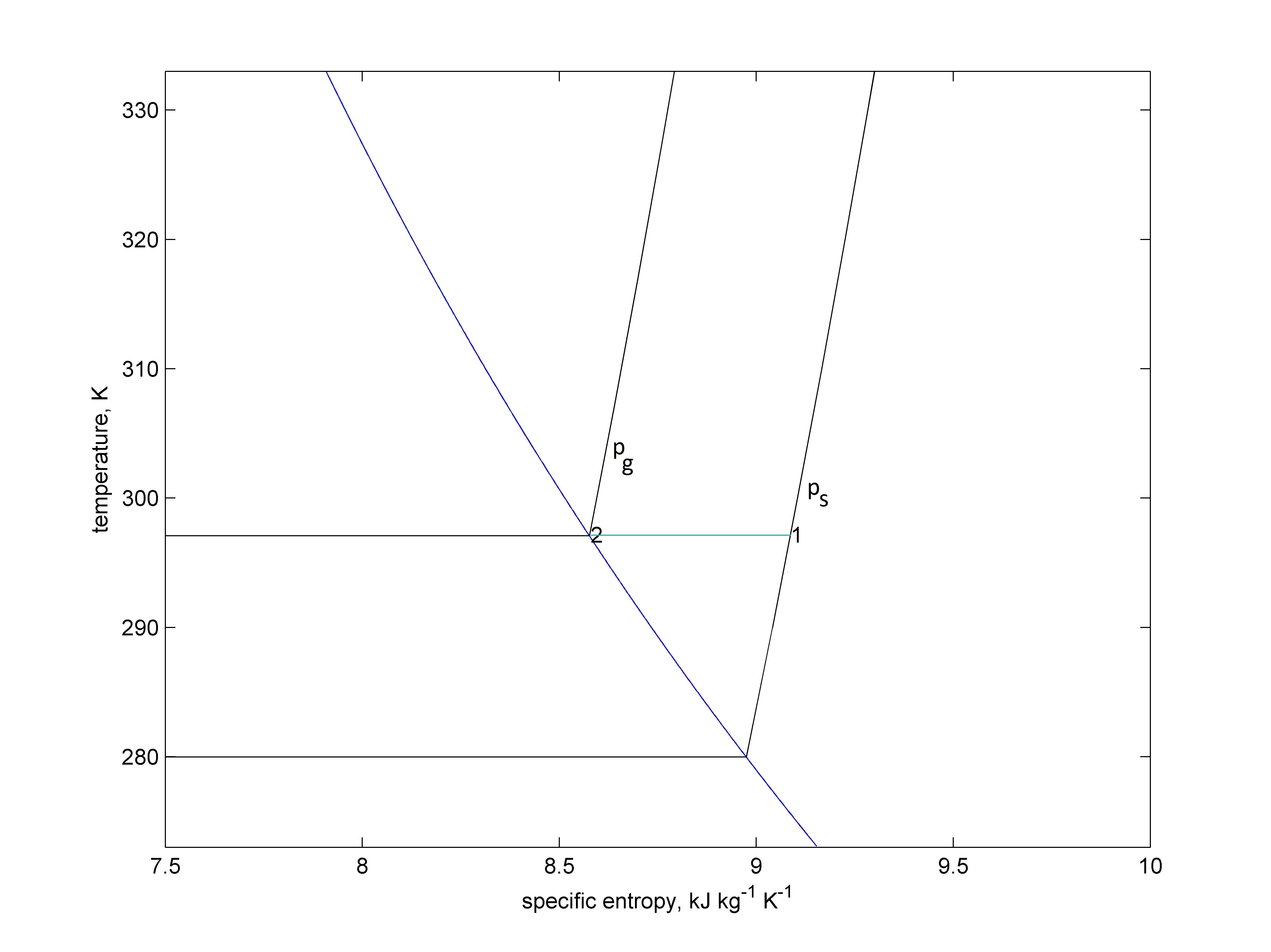
The dew point is the temperature to which unsaturated air must be cooled to initiate condensation . It is the point at which the first drop of dew is observed on a surface. Air at its dew point is said to be "saturated" with water vapour. At a given steam partial pressure, \(p_s\), the dew point can be read from steam tables as the corresponding saturation temperature.
The T-s diagram below shows locations of unsaturated air (#1) and saturated air (#2) at the same temperature. For symbol 1 the dew point is 280K whereas for point 2 it is equal to the actual temperature, about 295K.
Figure 1. The partial pressures in unsaturated air ( \(p_s\) at 1 ) and saturated air at the same temperature (\(p_g\) at 2). The blue curve represents saturated steam, the black curves
represent isobars. Specific entropy refers only to the vapour component of moist air
The wet-bulb temperature is achieved by a small sample of water in thermal equilibrium with its surroundings .
A thermometer normally records the 'dry bulb' temperature of an air stream. If however a separate bulb is wrapped with damp gauze, then water will evaporate away from the gauze when the surrounding air is not saturated with vapour. For the purposes of measurement thermal equilibrium is promoted by a
sling hygrometer
(or whirling hygrometer). The resulting cooling of the wet bulb depends on the relative humidity of the air stream, and for vigourous air flow rate yields "wet bulb temperature". The difference between wet and dry bulb temperatures enables relative humidity to be found from a psychrometric chart .
Let us consider calculation of the equilibrium at the wet bulb. The convective heat transfer into the water is equal to the rate of evaporative cooling. The controlling resistance is assumed to be in the gas-phase, so that the temperature at the water-air interface is equal to the bulk wet-bulb temperature, and the vapour pressure at the interface is the saturation pressure at the water-air interface. The driving force for convective heat transfer is taken as the temperature difference between bulk air and interface. The driving force for evaporative cooling is taken as the difference in steam pressures between bulk air and interface. The corresponding heat fluxes are,
Note that here t is the dry bulb temperature. (It is the custom to use temperatures on a two point scale, namely the Celcius scale, and this is indicated by the use of lower case t.) At equilibrium the heat fluxes sum to zero and the driving forces are related by the psychrometric constant ,
$$ \frac { p_s-p_g(t_{wet})} { t-t_{wet} } = (-1) \times A \times p $$
Parish and Putnam give the psychrometric constant for a sling hygrometer as ,
$$ A = 6.6 \times 10^{-4}+7.57 \times 10^{-7} \times t_{wet} \qquad psychrometric \; constant, \; t_{wet} > 0°C $$
So the true steam pressure, and thus all other quantities, follow from the reading of wet bulb temperature ,
$$ \boxed{ p_{s} = p_{g}(t_{wet}) - A \times p (t-t_{wet}) \qquad estimated \; steam \; pressure \qquad (5)}$$
A useful concept is the
enthalpy of moist air on the basis of 1kg of its dry component .
$$ H^* = \frac{enthalpy \; of \; dry \; air \; + \; enthalpy \;of \; steam}{mass\;of\;dry\;air\;only} $$
where t is in Celcius and the steam enthalpy \(h_s\) takes its datum as water at 0°C.
Example TZ010: Air at \(35^oC\) and a barometric pressure of \(p= 1.000 bar\) has a relative humidity of \(\phi=0.9\) . Calculate the specific humidity, \(\omega\) , the dew point, \(T_d\),
and the enthalpy term \(H^*\). Estimate the wet bulb temperature for a dry bulb temperature
of \(35^oC\) and 60% relative humidity.
Solution:
'Steam tables'
yield steam saturation pressure at \( 35^oC , \; p_g = 0.05629 bar\).
The steam partial pressure is: $$p_s = \phi \, p_g = 0.9 \times 0.05629 = 0.05066 bar$$
Tables show saturation pressure at 0.05066 bar: $$T_{dew} =33.1^oC$$
We now know steam partial pressure \(p_s\) and total pressure p so specific humidity is:
(This exceeds the maximum value, 0.021, on the psychrometric chart.) At 1, air is unsaturated at 0.05066 bar. The tables confirm that the sensitivity of enthalpy to pressure is confined to the fourth significant figure. So we take data from the row p = 0.05 bar. Interpolate between the saturation temperature ( \( 32.9^oC \; and \; 50^oC \)).
If the datum state is with moisture in the liquid phase and all species at zero celcius,
\begin{align}
H^* &= enthalpy \; in \; 1kg \; dry \; air \; + enthalpy \; in \; \omega \; kg \; steam \\
& = c_{p,a} T + \omega h_s \\
& = 1.005 \times 32.9 + 0.0332 \times 2565 = 118.2 kJ/kg(air)
\end{align}
Given that \(35^oC = 95^oF\), at 60% relative humidity a
pschrometric chart yields \(T_{wetBulb} \approx 83^oF = 28^oC\).
You can check the above at
our interactive Ts chart .
To obtain precise values, edit barometric pressure,
temperature, and relative humidity before pressing the "Calc & plot" button.
4. Air Conditioning - Equipment
Human comfort is related to both temperature and relative humidity. I describe a plant wherein(1) air is cooled to promote condensation and reduce humidity (2) the cooled air is reheated to a comfortable temperature .
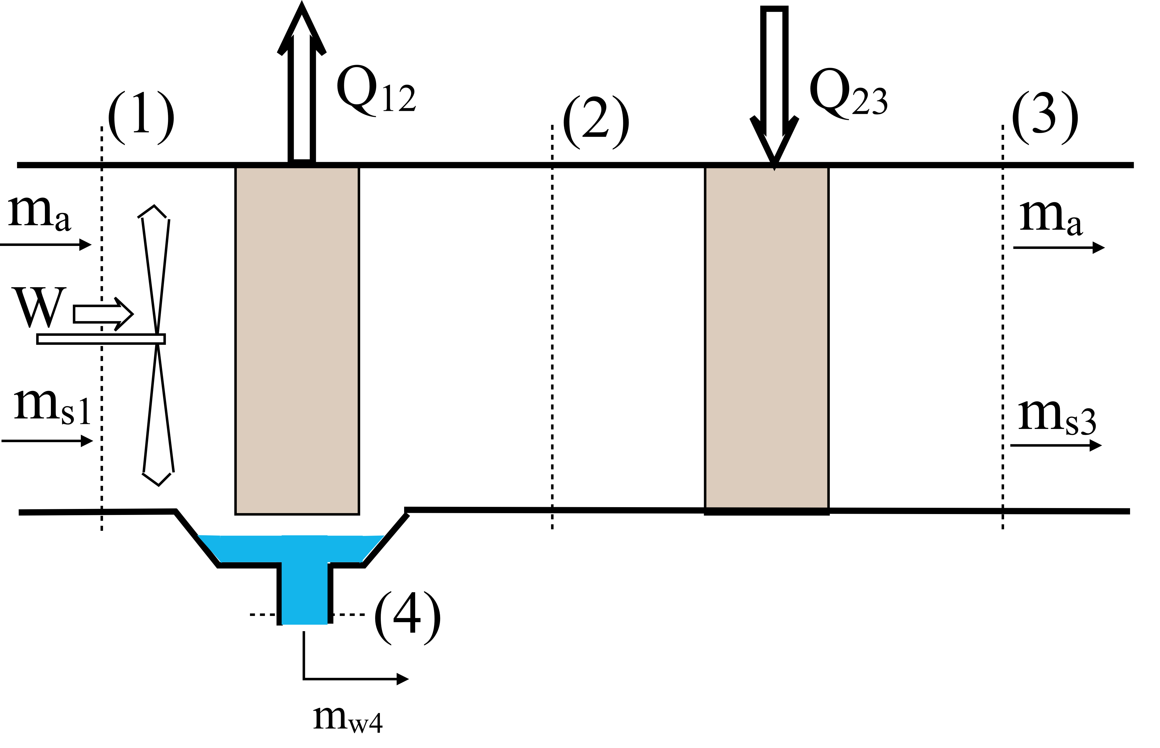
The air in the above example is both hot and humid. Humans find humid air particularly uncomfortable. The purpose of air conditioning is to both reduce temperature and reduce humidity. This is done firstly cooling the air to a temperature well below its dew point, so that some of the “steam” condenses. The temperature may well be then too cold, so that some reheating is needed. Rogers and Mayhew present a sketch of the equipment, redrawn as a block diagram below plus the T-s diagram.
Figure 2. Air Conditioning Plant. Gray rectangles correspond to heat exchange coils (Q12 and Q23)
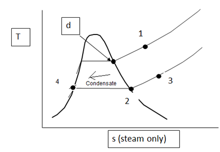
Figure 3. Process path for air conditioning plant, shown on a Ts plot
Let us follow the transit of moist air through the Ts diagram. Air is cooled from 1-to-d-to-2. Point d indicates the dew point; beyond here further cooling causes condensation. A moisture trap at the heat exchanger exit separates moist air from condensate. If the two are at thermodynamic equilibrium then air temperature and condensate temperature are equal; \(T_2=T_4\). Note that total pressure is constant throughout the plant, 1-d-2-3. From 1-to-d there is no condensation so the ratio of steam and air mass (specific humidity, \(\omega\)) remains constant, as does steam partial pressure, \(p_s\). Condensation from d-to-2 changes both \(p_s\) and \(\omega\) the air is saturated so that \(\phi=1\) and \(p_s = p_g\). The temperature at 2 would be uncomfortably cold, necessitating the reheating and from 2-to-3 (again with no change in steam partial pressure or specific humidity). Notice that at input 1 and required condition 3, humidities are specified as relative humidities.
Example TZ020: Consider the plant shown on Figure 2. Conditioned air is produced at a relative humidity of 55% , a temperature of \(20^oC\), and a volumetric flow rate of \( 30m^3\,min^{-1}\) (of moist air). Use the previously calculated conditions for the plant inlet, including a barometric pressure of 1 bar. Find all mass flows.
Solution:
Recall from the previous example,
$$ \omega_1 = 0.0332 $$
At outlet
'steam tables'
give the saturation pressure as \(p_{g3}(20^oC) =0.02337 bar\)
\begin{align*}
p_{s3}=&\phi_3 p_{g3}= 0.55 \times 0.02337=0.01285 bar \\
\omega_3=&0.622 \times \frac{0.01285}{1-0.01285}=0.0081
\end{align*}
Use the Ideal Gas Law to get the mass flow rate of dry air and also use the partial pressure
of dry air, \(p_a=p-p_s\) (Gibbs Dalton)
\begin{align*}
\dot{m}_a=&\frac{p_a \, \dot{V}}{R_a \,T}= \frac{(1-0.01285) \times[100] \times 30)}{0.287 \times (273+20)} = 35.22\,kg\,min^{-1} \\
\end{align*}
Dry air does not condense so its mass flow rate is constant throughout the plant
The latter is because no steam condenses between 2 and 3.Total mass flow is found by simple addition of the steam and air components. The mass
flow of condensate is the differentce in steam flows.
The difference in steam mass flows (in - out) is equal to the rate of production of condensate. I shall write this is
\begin{align*}
\dot{m}_{w4} & =\dot{m}_a(\omega_1-\omega_3)=35.22\times(0.0332-0.0081)= 0.884\,kg\,min^{-1} \qquad or \\
\dot{m}_{w4} & = \dot{m}_{s1} - \dot{m}_{s2} = 1.169-0.285 = 0.884\,kg\,min^{-1}
\end{align*}
We now turn our attention to the energy balance. The necessary assumptions are as follows.
Steady conditions - no heat transfer appears as a change in temperature and internal energy.
Ignore kinetic energy and potential energy terms in SFEE.
Thermal equilibrium between streams \#2 and \#4.
The fan work might (or might not) be ignored.
The total pressure, that is \(p=p_a+p_s\), is constant. This means that from 2-to-3, where no condensation occurs and the specific humidity, that is the mass ratio \(m_s/m_a\), is constant, then the partial pressures of dry air and steam are constant .
Under steady conditions, there are four reasons why pressure might change along a conduit. Friction causes a reduction in pressure. Heating will accelerate fluid (because density is reduced) and again pressure is reduced as pressure energy is converted to kinetic energy. Conversely cooling will decelerate the fluid and increase pressure. Condensation, by virtue of removal of material from the gas phase, also decelerates fluid and causes pressure to increase. All these effects are very small and for educational purposes at least can be ignored.
We can also recap Physical Principles :
First law in form of Steady Flow Energy Equation
Gibbs Dalton law implies that enthalpy of moist air = dry air enthalpy + steam enthalpy
Law of mass conservation implies amount of condensate = change in amount of steam.
The Gibbs-Dalton law allows us to "imagine" dry air and steam as being conveyed in separate pipes. Dry air is conveyed as streams a1, a2 and a3 whereas steam is conveyed in streams s1, s2 and s3. A special multi-stream version of the SFEE then applies.
\begin{equation}
\boxed{ \dot{Q}+\dot{W}=\sum (\dot{m}_j h_j)_{out} - \sum (\dot{m}_k h_k)_{in} \qquad (7)}
\end{equation}
On Figure 2, the multistream SFEE would be used for the heater (system boundary cutting streams 1, 2, and 4) and
the cooler (system boundary cutting streams 2 and 3). Stream 4 carries water in its liquid phase.
A worked example will use the previous inlet conditions.
You must have a consistent datum for all moisture enthalpies. Use the same steam tables, chart or database for s1, s2, s3 and w4.
Example TZ030 – Consider the plant shown on Figure 2. If \(30 \, m^3 \, min^{-1}\) of (moist) air is required, estimate the necessary rate of cooling
Solution:
In the following ignore fan power, changes in potential and kinetic energy and assume constant total pressure throughout the plant.
Refer to the plant diagram in Figure 2 and T-s diagram in Figure 3 (note that entropy is that of the water component only).
Recall the following estimates from Examples TX010 (inlet at \(35^oC, 90\%\) relative humidity)
and TZ030.
$$ \qquad p = 1.00bar \; and \qquad p_{s1} = 0.05066 bar \qquad p_{s2}=p_{s3} = 0.01285bar \qquad steam \; partial \; pressures $$
$$ \qquad \omega_1 =0.0332 \qquad \omega_2=\omega_3 = 0.0081 \qquad specific \; humidities $$
$$h_{s1} = 2565 kJ kg^{-1} \qquad steam \; enthalpy $$
$$ \qquad \dot{m}_a = 35.22 kg \; min^{-1} \qquad mass \; flow \; rate \; of \; dry \; air $$
Start at 2 where (see Ts diagram, Figure 3) air is saturated and \( p_{g2}= p_{s2}=p_{s3}=12.85 \; mbar\) lies between 10 and 15 mbar. Linear interpolation the saturated steam data in
'steam tables' yields,
\begin{align*}
T_2 &= 7 + (13-7)\times(12.85-10)/(15-10) = 10.4^oC \\
h_{s2} &= 2514 + (2525-2514)\times (12.85-10)/(15-10) = 2520 kJ kg^{-1} \\
h_{w4} &= 44 kJ kg^{-1}
\end{align*}
The multi-stream version of the SFEE, Equation 7, is applied to the control volume bounded by 1, 2, 4. At 1 treat steam and dry air as separate streams (likewise at 2). Then,
\begin{align*}
\dot{Q}_{12}=&(\dot{m}_a \, h_{a2} + \dot{m}_{s2} \, h_{s2}+\dot{m}_{w4})-(\dot{m}_a \, h_{a1}+\dot{m}_{s1} \, h_{s1}) \\
\dot{Q}_{12} =&\dot{m}_a c_{pa} (T_2-T_1)+\dot{m}_a \omega_2 \, h_{s2} - \dot{m}_a \omega_1 \, h_{s1} + \dot{m}_{w4} \, h_{w4}
\end{align*}
On the second line above the enthalpy of air follows from heat capacity, hence \(h_a=c_pT\). The mass flow rate of steam is the produce of dry air flow rate and specific humidity, \(\dot{m}_s = \dot{m}_a \omega \),
We also need the heat addition from 2 to 3. All conditions at 2 are known and at 3 (using \(T = 20^oC\) and the row \(p_s = 0.01 bar \) on the superheated version of the steam tables) \( h_{s3} = 2539 kJ kg^{-1}\).
This is correct because there is no condensation and hence \(\dot{m}_{s3} = \dot{m}_{s2}\). Again, note identical specific humidities, \( \omega_2=\omega_3\). Assuming that a refrigeration plant is used for the cooling demand, some of the heat rejected from the condenser might be appropriate for the heating demand, \(Q_{23}\).
The above calculation can be repeated, with some loss of precision, using paper versions of the psychrometric charts,
our own interactive version, or our interactive Ts chart . Using the latter,
At point 1: set barometric pressure of p=1.000bar, relative humidity of ϕ=0.9, temperature = 35 deg. C.
Press "calc and plot". Note \(H^*_1=120.3kJ/kg, \; \omega_1=0.03319\). Plot as symbol with label 1. Plot the isobar.
At point 3: set relative humidity of ϕ=0.55, temperature = 20 deg. C. Set label to '3'.
Press "calc and plot". Note \(H^*_3=40.7kJ/kg, \; \omega_3=0.00811 \). Plot the isobar.
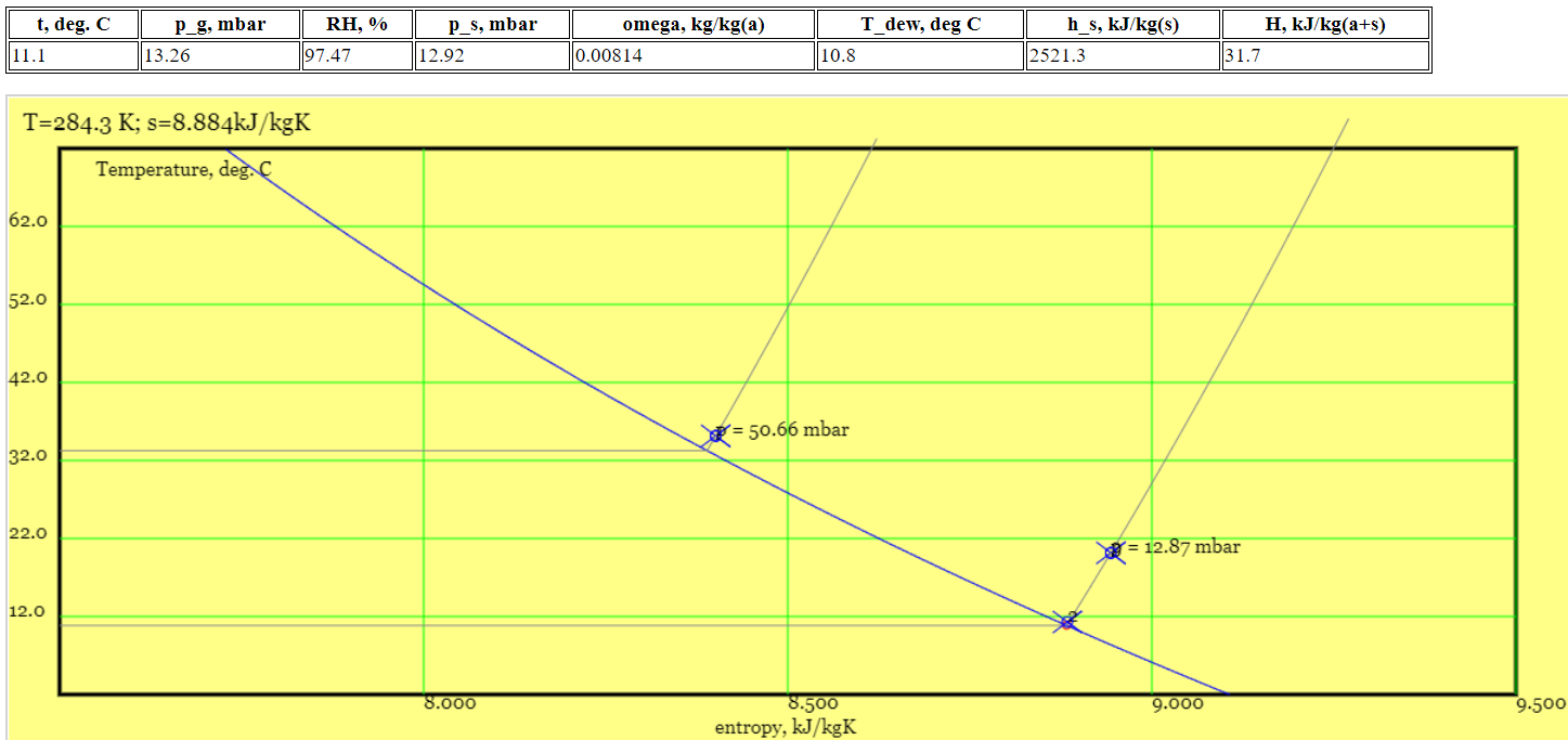
At point 2: by eye, click at the intersection point between the 12.87mbar isobar and the saturation line.
Note \(H^*_2=31.2kJ/kg, \; \omega_2 = 0.00811 \; T_2=10.7^oC \; \phi_2=1\) - this is not quite a perfect match. Set label to '2' and click 'plot symbol'.
Use the air mass flow rate and water flow rate calculated previously. Take the water enthalpy as \(4.2 \times t\), assuming a specific heat capacity of \( 4.2 kJ/kgK \) and noting that the values are roughly in line with steam tables. Then the cooling demand follows,
Figure 4. Use of online plotter to size an airconditioning plant. The table shows data at point 2.
6. Psychrometric Charts
Many pschrometric properties and processes can be plotted on paper charts.
The psychrometric chart offers an alternative presentation to the T-s diagram. It is well known by practitioners working in
with air conditioning and the built environment. To simplify the large amount of information conveyed by the paper versions I
show simplified forms in Figure 6. The diagrams are downloaded from my
interactive version of the psychrometric chart .
Part (a) shows a simple version of the chart - a point of interest is defined by dry bulb
temperature on the x-axis and specific humidity on the y-axis. At any given temperature the specific humidity has a saturation value - above which vapour will form fog or condense. At point 1 on Figure 6a the dry bulb temperature is 32°C, the specific humidity is about 0.016 and air would be saturated if the specific humidity were raised to about 0.030. The curve bounding the white and blue zones describes the upper limit of specific humidity, and the white area is a "no-go" zone -
only the blue zone is usable. Within the "blue zone", all other properties of state can be calculated from temperature and specific humidity- on our
interactive chart this is done by clicking the point of interest. On paper graphs one must interpolate between lines or curves corresponding to
the required property.
Figure 6b shows three curves of constant relative humidity. For example, along the 67% curve, the specific humidity is approximately (but not exactly) 67%
of the saturation value at the same temperature. Figure 6c shows two lines of constant wet-bulb
temperature. If we follow these along to the saturation curve (RH=100%) we find equal
wet bulb and dry bulb temperatures. There are also two lines of constant
total specific enthalpy.
(a) (b)
(c)
Figure 6. Use of the Psychrometric chart.. (a) unused chart, with the "no-go" zone shaded white and all properties at the indicated point calculable from dry bulb temperature (x-axis) and specific humidity (y-axis) (b) curves of constant relative humidity
(c) two lines of constant total specific enthalpy (near bottom) and two lines of constant wet bulb temperature (near top)
Hyndman discusses
paper versions of the psychrometric chart
. The dry bulb temperature is listed along the x- axis and specific humidity (or "humidity ratio") along the right hand y axis. Separate curves of constant relative humidity \(\phi\)
extend from bottom left edge to top right edge. The curve for \( \phi=100\%\) bounds the plot area.
The diagonal lines that extend from bottom left to top right represent lines of constant
wet bulb temperature. Some psychrometric charts are modified to include vapour pressure and the
enthalpy term \(H^*\) - a more detailed version is
here .
Figure 7 represents the problem from Section 5, concerning cooling, condensation and reheating to
condition air. The cooling has two sub-processes. The sub-path from 1 to saturation at d is sensible cooling along the
horizontal line of constant specific humidity, \( \omega = 0.003318 \). There is then is appreciable
loss of latent energy along the saturation line from poind d to point 2.
The reheating process avoids phase change and follows the horizontal line \( \omega = 0.00811 \).
Values found from the interactive chart match those in Section 5 (remember first of all to reset the barometric
pressure to 1000 mbar).
Figure 7. Psychometric chart showing airconditioning process considered in section 5. Cooling is mapped from 1 to the saturation line (constant specific humidity), down the saturation line to 2. Heating is at constant specific humidity from 2 to 3.
Adiabatic Mixing
It is sometimes mandatory to mix conditioned air with fresh air from outside a building, see for example Dincer and Rosen . The process is, for practical purposes, adiabatic. The process of mixing lends itself to the use of pyschrometric charts. If streams 1 and 2 are merged to form stream 3 then the following balances ensue.
The penultimate and ultimate balances yield the mixture's specific humidity \(\omega_3\) and total enthalpy \(H^*_3\). When paper charts are used, lines of constant \(\omega\) and \(H^*\) intersect to yield the condition of the mixed stream.
Figure 8 illustrates steps in the calculation. Specified temperatures and relative humidities yield the states prior to mixing (part a)- on the paper version of the chart one would find the intersection of the curves of constant \( t \; and \; \phi \). The specificy humidity ( \( \omega \) ) and enthalpy ( \( H^* \) ) of the mixed stream are calculated and then yield its state.
Figure 8. Psychometric chart showing mixing of two streams (a) states of two streams, located at the intersection of vertical lines of constant temperature and curves of constant relative humidity (b) location of steam 3, using lines of constant specific humdity ( \( \omega \) ) and constant enthalpy ( \( H^* \) ). Values of \( \omega, H^* \) were computed from material and energy balances.
Example TZ040: Two streams of known dry bulb temperature, volumetric flow rate and relative humidity are mixed adiabatically. Estimate the properties of the resulting mixed stream. The values before mixing are,
\begin{align}
t_1 &= 14°C \qquad \dot{V}_1 =50m^3/min \qquad \phi_1= 100\% \\
t_2 &= 32°C \qquad \dot{V}_2 = 20m^3/min \qquad \phi_2=60\%
\end{align}
Solution:
From the chart (see Figure 8a), specific humidity, specific volume and enthalpy are,
A cooling tower reduces the temperature of water by means of evaporative cooling.
The exploitation of evaporative cooling should result in a far smaller demand for electricity than that of a refrigeration plant, limited to the
"parasitic power" of fans and pumps.
Descriptions and photographs of the operation of a cooling tower are available at
commercial websites . In the forced draft tower, a fan pushes air upwards whereas water flows downwards over packing . Hence the tower is a countercurrent heat and mass transfer operation. In older units wooden slats were used as packing whereas now premanufactured modular packs are employed. The purpose of the pack is expose a large surface area of water to the air stream.
Energy balance and exit conditions
An energy balance on the tower yields the state of the exit air and the cooling demand. Let us ignore evaporative losses and treat the mass flow rate of water as constant. Let 1 indicate the point of air entry (base of tower) and let 2 indicate the point of air exit (top of tower). Use the Steady Flow Energy Equation on the water and air
streams to find rates of heat transfer.
\begin{align}
\dot{Q}_{air} &= \dot{m}_a (H^*_2 - H^*_1) \qquad \qquad heat \; transfer \; to \; air \\
\dot{Q}_{water} & = (-1) \times \dot{m}_w c_{pw} (t^{water}_2 - t^{water}_1 ) \qquad heat \; transfer \; to \; water \; = \; cooling \; demand \\
\end{align}
(the factor of (-1) deals with counterflow, making 2 the point of water inlet at the top of column.) Assuming steady conditions and an adiabatic tower, and ignoring changes in kinetic energy and potential energy, the heat transfers to air and water streams should sum to zero.
$$ \dot{Q}_{air} = (-1) \times \dot{Q}_{water} $$
On rearrangement, the exit enthalpy of air becomes
$$ \boxed{ H^*_2 = H^*_1 + \frac{\dot{m}_w c_{pw}}{\dot{m}_a}(t^{water}_2 - t^{water}_1 ) \qquad air \; exit \; enthalpy \; (8) } $$
At this point we have not specified in full the state of the exit air - we know only that it lies somewhere
on a line of constant enthalpy, and that the specific humidity is greater that its inlet value. In the next section Equation 8 defines the
air operating line .
Example TZ050: Water at 30°C is fed to the top of a cooling tower and is to be
cooled to 25°C. Air is supplied to the base of the tower at a flow rate twice that of the water.
The air is at a dry bulb temperature of 20°C and a wet bulb temperature of 10°C. Estimate the heat removal per kilogram of water, and the enthalpy of the air
at inlet and outlet.
Solution:
Apply SFEE to the water stream,
\begin{align}
\frac{\dot{Q}_{water}}{\dot{m}_w} & = (-1) \times c_{pw} (t^{water}_2 - t^{water}_1 ) \\
&= (-1) \times 4.18 \times (25-30) = -20.9 kJ/kg
\end{align}
From the psychrometric chart, the enthalpy of inlet air is,
$$ H^*_1 = 28.73 kJ/kg \qquad at \; 20°C\;(dry\;bulb)\;10°C \; (wet \; bulb ) $$
Apply SFEE to the air stream, noting that the air mass flow is twice that of the water,
\begin{align}
\dot{Q}_{air} = (-1) \times \dot{Q}_{water} = 20.9 kJ/kg \times \dot{m}_w \\ \\
H^*_2 = H^*_1 + \frac {\dot{ Q}_{air}}{\dot{m}_a} = 28.73 + \frac{20.9 kJ/kg \times \dot{m}_w }{2 \dot{m}_w } = 39.18kJ/kg
\end{align}
The height of the tower
Merkel's model of a cooling tower is frequently cited. Equations for sensible and evaporative heat transfer are combined elegantly into a
a single expression that works adequately with air and water. (This might well not be the case
for other combinations of gas and liquid.) Consider the interfacial boundary between the water and the air (Figure 9a, on which packing is shaded brown and water blue). On the air-side of this interface
the air is treated as saturated with water vapour and at the water temperature. Thus Figure 9b shows two characteristics. The red line shows the air enthalpy at any
point, \(H^*\), plotted against the corresponding water temperature, \(t^{water}\) (see the previous enthalpy balance equation). The black curve shows the interfacial air enthalpy, \(H^*_i\), at given water
temperature (this equals the saturation enthalpy on the pyschrometric chart, at the water temperature and a relative humidity of 100%).
(a) (b)
Figure 9 Role of enthalpy (a) sketch of a small control volume of packing \( \delta V\) with profile (in red) of enthalpy from interface to bulk air;
packing is shaded brown and water is shaded blue
(b) air operating line (red) and saturation curve (black)
The driving force for total heat transfer from the water to the air is the difference in enthalpy
between the interfacial air and the bulk air.
To consider how the enthalpy driving force works,
consider the local heat transfer per unit volume in a very small part of the column, in which
there is minimal variation in \(t^{water}, H^*, \; or \; H^*_i\). For example, in Figure 9a the dotted line could bound volume \(\delta V\) inside which the heat transfer rate from
the interface to the bulk air is \( \delta \dot{Q}_{air} \).
\begin{align*}
\frac { \delta \dot{Q}_{air} }{\delta V} &= K \qquad a \qquad ( H^*_i - H^* ) \qquad volumetric \; heat \; transfer \\ \\
\frac{kJ}{m^3 s} &= \frac{kg}{m^2 s} \; \frac{1}{m} \qquad \frac{kJ}{kg}
\end{align*}
$$ $$
where K is a mass transfer coefficient, \(H^*\) is the bulk air enthalpy, and \(H^*_i\) is the interfacial enthalpy evaluated from the water temperature
\( t^{water} \) and at relative humidity \( \phi=1 \). Term a is the area of exposed surface per unit volume of the column - it has units of \( \frac{m^2}{m^3} = m^{-1} \).
Integration of the above yields the required volume of packing, V.
$$ K a V = \frac { \dot{Q}_{air}}{( H^*_i - H^* )_{HM}} \qquad yields \; packing \; volume $$
where HM indicates a
harmonic mean
enthalpy difference (see appendix for full integration ). To obtain the heat transfer term recall from the previous heat balances that
\( \dot{Q}_{air} =
(-1) \times \dot{Q}_{water} = \dot{m}_w c_{pw} (t^{water}_2 - t^{water}_1 ) \). Substitute into the above to find,
The term on the left hand side is known as the tower characteristic . A further useful parameter is the loading factor, the mass flux density of the water flow \(\dot{m}_w/A\). The tower manufacturer will have measured optimum loading factors for different operating conditions - too high a loading factor will cause high fan power and in some instances flooding, whereas low factors result in excessive cost of equipment and land. The loading factor allows estimates of tower height. One should also be aware of potential problems with flow distribution and column flooding, plus estimating the power demand of pumps and fans - issues well beyond the scope of these notes.
Worked Example
The following is adapted from a report by
Leeper, available online.
Example tz060: A cooling column is operated with inlet air supplied at a wet bulb temperature of 23.8°C and a loading factor of
\(1.86 kg/m^2s\). (The loading factor is the mass flow rate of water per unit of tower cross section.
) The water flow rate is 18.6kg/ s. Other conditions and parameters are,
\begin{align}
\dot{m}_w & = 1.36 \dot{m}_a \qquad mass \; flows \\
t^{water}_1 &=48.3°C \qquad \qquad inlet \; water \; temperature \; at \; top \; of \; tower \\
t^{water}_2 &=31.7°C \qquad \qquad outlet \; water \; temperature \; at \;base \; of \; tower \\
Ka &= 0.445 kg/m^3 s
\end{align}
Estimate the height of the tower, its cross sectional area and the cooling load.
Figures and assumptions: See Figure 9. No changes in kinetic or potential energy, steady conditions, adiabatic tower, ignore energy
addition from pumps and fans.
Air condition: Only the wet-bulb temperature is given at inlet, but the lines of constant enthalpy and constant wet-bult temperature are very close.
Thus for a given wet-bulb temperature variations in a second parameter have little influence on H*. If \( \phi=1 , \; t_{wet}= 23.8°C\), you can use the
interactive version of the psychrometric chart to find
$$ H^*_1 \approx 71.38 kJ/ kg $$
Energy balance over the air and water streams give the air operating line. The second air point is,
$$ H^*_2 = H^*_1 + \frac{\dot{m}_w c_{pw}}{\dot{m}_a}(t^{water}_2 - t^{water}_1 ) $$
$$ H^*_2 = 71.38 + 4.18*(30/1.8)*1.36 =166.1kJ/kg $$
Harmonic mean enthalpy difference: Several authors have carried out integration by the four point Tchebycheff method.
We find conditions at water temperatures of 31.7+fraction * (48.3-31.7)°C where fraction is 0.1, 0.4, 0.6 or 0.9.
(Strictly speaking we should use [ 0.102673, 0.406204, 0.593796, and 0.897327] .)
This is tablulated below.
fraction
\(t^{water}\).°C
H*, kJ/kg(air)
H*_i , kJ/kg(air)
H*_i-H*, kJ/kg (air)
0
31.67
71.40
0.1
33.33
80.88
118.46
37.59
0.4
38.33
109.30
152.69
43.39
0.6
41.67
128.25
180.54
52.29
0.9
46.67
156.68
232.2
75.53
1
48.33
166.15
Example. Note the range is 48.3-31.7= 16.6°C. If fraction =0.4,
\begin{align*}
t^{water} &= 31.7 + 0.4 \times 16.6 = 38.3°C \\
H^* &= 71.4 + 0.4 \times (166.2-71.4) = 109.3 kJ/kg \\
H^*_i &= f(38.3, \phi=1) = 152.7 kJ/kg \\
H^*_i-H^* &= 152.7-109.3 = 43.4 kJ/kg
\end{align*}
The values of "fraction" correspond to a four-point quadrature ( see appendix ). The saturation enthalpy can be found with
interactive version of the psychrometric chart,
even when plot limits are exceeded.
Find the harmonic mean of the enthalpy differences:
$$ (H^*_i-H^*)_{HM} = \frac{4}{ 1/37.59 + 1/43.39 + 1/52.29 + 1/75.53} = 48.8 kJ/kg $$
Find the (dimensionless) tower characteristic:
$$ \frac{KaV}{\dot{m}_w } = \frac { c_{pw}(t^{water}_2 - t^{water}_1) }{( H^*_i - H^* )_{HM}} \qquad tower \; characteristic $$
$$ \frac{KaV}{\dot{m}_w } = \frac { 4.18(48.3- 31.7)}{ 48.8 } = 1.428 \qquad vs \;1.408\; (Leeper) $$
Find the tower height (z): Note first the simple geometric relationship \(V=zA\), where A is cross
sectional area. For a given loading factor and mass transfer coefficient,
$$ \frac {\dot{m}_w } {A} = 1.86 kg/m^2 s \qquad (given) $$
$$ Ka = 0.445 kg/m^3 s \qquad (given) $$
Then
$$ z = tower \; characteristic \times \frac {\dot{m}_w } {A} \times \frac{1}{Ka} $$
$$ z = 1.428 \times 1.86 kg/m^2 s \times \frac{1}{0.445 kg/m^3 s} = 6.0 m \qquad vs \;6.0m(Leeper) $$
A more rigorous and detailed discussion of Merkel theory is presented here. Refer to Figure 9. Write expressions for the
convective heat transfer per unit volume and evaporative mass transfer per unit volume, both transfers in the direction from the interface to bulk air (I shall drop the "air" subscript here). Note that for the
mass flux the driving force is difference in mass concentration, kg(steam) per cubic metre of moist air, and for dilute mixtures of vapour-air
the mass concentration is approximately equal to the product of air density and specific humidity, \( c_s \approx \rho_a \omega \).
$$ \frac{\delta \dot{Q}_{conv}}{\delta V} = \alpha a (t_i-t) \qquad \qquad (A1) $$
$$ \frac{\delta\dot{m}_{evap}}{\delta V} \approx K' a \rho_a (\omega_i -\omega ) \qquad \qquad (A2) $$
where a is the exposed surface area of water per unit volume of packing, \( \alpha \) is the convective heat transfer coefficient and K' is termed the mass transfer coefficient . Temperature t and specific humidity \( \omega \) refer to conditions in the bulk air .
Now consider the profiles of temperature and mass concentration in the boundary layer. Let y be the perpendicular distance
from the interface to a point of interest, and let us describe the profiles with a function g(y) and the boundary layer thickness \( \delta \),
\begin{align}
\omega (y) &= \omega_i - g(y ) ( \omega_i - \omega ) \qquad 0 \le y \le \delta \qquad g(0)=0 \qquad g(\delta)=1\;\qquad humidity \; profile \\
t(y) &= t_i - g(y ) (t_i - t) \qquad 0 \le y \le \delta \qquad temperature \; profile
\end{align}
where the same function, g(y) and the same boundary layer thickness \(\delta\) apply to both heat and mass transfer. This equality is accepted
as a fair approximation for air and steam but might not be so for other gas mixtures
At the interface, y=0, there is minimal turbulence and heat transfer can be estimated, temporarily, by the Fourier law. Likewise mass transfer
can be estimated by Fick's First Law.
where D is the mass diffusivity and air density has been treated as constant. Use the function g(y) to obtain the gradients of temperature and humidity.
$$ \frac{\delta \dot{Q}_{conv}}{\delta V} = +\lambda \frac{dg(y)}{dy} (t_i - ) a \qquad (at \; y=0) $$
$$ \frac{\delta\dot{m}_{evap}}{\delta V} \approx +D \rho_a \frac{d g(y)}{dy } ( \omega_i - \omega ) a\qquad (at \; y=0) $$
In passing, compare these with equations A1 and A2: for the heat transfer coefficient \( \alpha = \lambda \frac{dg(y)}{dy} \) and for the
mass transfer coefficient \( K' \approx D \rho_a \frac{d g(y)}{dy } \).
Let us treat the evaporative heat transfer as the product of mass flux and the specific enthalpy of steam, \(h_s\),
$$ \dot{Q}_{evap} \approx \dot{m}_{evap} h_s $$
where \(h_s\) will for the current purposes be treated as independent of temperature. Then the total volumetric heat transfer is
$$ \frac{\delta \dot{Q} }{\delta V} = \frac{dg(y)}{dy} a \times ( \lambda (t_i - t ) + D \rho_a ( \omega_i - \omega ) h_s) \qquad (A3) $$
For the specific instance (again) of air-water, the Lewis number is approximately equal to one. This means that mass and thermal diffusivities are roughly equal, or
$$ D \approx \frac{\lambda}{\rho_a c_{a} } \implies \lambda \approx D \rho_a c_{a} $$
and therefore we need use only one of the diffusivities in Equation A3, by convention the mass diffusivity
$$ \frac{\delta \dot{Q} }{\delta V} = ( \frac{dg(y)}{dy} D \rho_a) \times a\times ( c_{pa} (t_i - t_{bulk} ) + ( \omega_i - \omega_{bulk} ) h_s) $$
The first group in brackets will be replaced with a new mass transfer coefficient, Rather than mass concentration, K implies that specific humidity is the driving force.
Let us ignore the change in sensible enthalpy, \(c_{ps}(t_i-t) \) ) so that \(h_s\) is constant and the total specific enthalpies are ,
$$ H^* = c_{pa} t + \omega h_s \qquad H^*_i \approx c_{pa} t_i + \omega_i h_s $$
The total heat transfer becomes,
$$ \frac{\delta \dot{Q} }{\delta V} = K a (H^*_i-H^*) $$
Substitute the heat balance, \( \delta\dot{Q} = \dot{m}_w c_{pw} \delta t \) so that
\begin{equation}
\boxed{
\frac{KaV}{\dot{m}_w } = \int^2_1 \frac { c_{pw}dt }{( H^*_i - H^* ) } \qquad (A4)
}
\end{equation}
This is the classic Merkel Equation.
I have reintepreted the RHS in the main notes as the quotient of (cp * temperature change) and
a harmonic mean enthalpy difference. Define dimensionless temperature in the range from 0 to 1 as
$$ \theta = \frac{t-t_1}{t_2-t_1} \implies d\theta = (t_2-t_1)dt $$
then the Merkel Equation becomes,
$$ \frac{KaV}{\dot{m}_w } = c_{pw} (t_2-t_1) \int^1_0 \frac { dt }{( H^*_i - H^* ) } $$
and the right hand side is the harmonic mean enthalpy difference .
Comments on the Integration Quadrature
In Example TZ060 the following equal-weighted quadrature was used to integrate in the range [0,1].
I believe the simplicity of the quadrature renders it useful for educational purposes and first estimates. However for professional purposes more
attention is needed to the accuracy of integration. An example of the quadrature's use for cooling towers is given
here and elsewhere online. However, I could not find any source for this information that presented underlying theory and tabulated quadrature point locations for different numbers of points. The closest was the use of 5, 6 and 7 point log-Tchebycheff quadratures for velocity traverses
in air ducts, widely available online , e.g. from an extract from
Legg's book on Air Conditioning System Design".
I tested the quadrature against the analytical solution to \( f(\xi) = exp (k \xi) \), with \( k = 0.2, 0.5, 1,2,3,4,5,6,7 \). The smallest error was
0.0003% (k=1) and the largest was 0.9% (k=4). (Identical errors are found for exponential decay, \( f(\xi) = exp (-k \xi) \).)